Day100 Deep Learning Lecture Review - Lecture 17 (1)

November 12, 2024 7 minute read

Understanding Conformal Prediction: Concepts, Applications, Marginal Coverage, and Recipes In Detail

Conformal Prediction

Unlike traditional point predictions, conformal prediction generates prediction regions—sets of predictions for classification tasks and intervals for regression tasks. These regions are guaranteed to encompass the correct outcome with a user-specified confidence level, provided that the framework’s conditions are satisfied.

What is Conformal Prediction?
- At its core, conformal prediction transforms traditional machine learning predictions into a format that includes uncertainty measures.
- This framework builds on the assumption that data points in the calibration set (used for conformal prediction) and the test set are exchangeable, meaning they come from the same distribution.

Key Outputs

Prediction Sets (Classification): For classification tasks, the model outputs a set of possible labels rather than a single label. For example, instead of predicting “cat,” the prediction might include {“cat,” “dog,” “rabbit”}. This set is guaranteed to include the correct label with high probability.
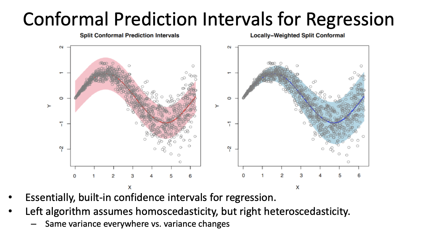
Prediction Intervals (Regression): For regression tasks, conformal prediction provides an interval (e.g., [4.2, 5.8]) that is statistically guaranteed to include the actual value with the specified confidence level (e.g., 90%).

Confidence Level ($\alpha$)
- By setting $\alpha$, we define the algorithm's error rate we’re willing to tolerate.
  $1-\alpha \leq \textbf{P}(Y_{test} \in C(X_{test})) \leq 1-\alpha +\frac{1}{n+1}$
- For example
  - $\alpha = 0.05$: The system guarantees that the prediction will be correct at least 95% of the time.
  - $\alpha = 0.1$: The prediction is correct at least 90% of the time.
- Smaller $\alpha$ values lead to larger prediction regions, which means wider intervals in regression or larger sets of labels in classification
- This trade-off between specificity and certainty is key to understanding and applying confromal prediction effectively.

How Does Conformal Prediction Work?

Two subsets of Conformal Prediction workflows
- Calibration: A subset of the data, separate from the training and test sets, is used to compute thresholds. This calibration set ensures that the predictions align with the desired confidence level.
- Prediction: Using the calibrated thresholds, the model outputs prediction regions for unseen data. These regions are dynamically adjusted based on the characteristics of the data and the uncertainty associated with each prediction.
Standard assumptions
- We have a pre-trained model for a prediction task.
  - Classification or regression
- He have a heuristic notion of uncertainty from the pre-trained model.
- We have a small amount of additional calibration data that was not used for training and is separate from test data.
- We have a nonconformity measure used to produce prediction regions.
Nonconformity measure
- A critical aspect of conformal prediction is the nonconfomity measure, which quantifies how “strange” or “unexpected” a new data point is relative to the calibration set.
- Higher nonconfomity scores indicate greater uncertainty.
- The choice of nonconformity measure can significantly affect the quality of prediction regions.
Quantiles and Thresholds
- Conformal prediction uses quantiles to define the cut-off for prediction regions.
- For instance, in classification, the algorithm includes all labels whose scores fall within a certain quantile threshold, ensuring that the prediction set captures the desired confidence level.
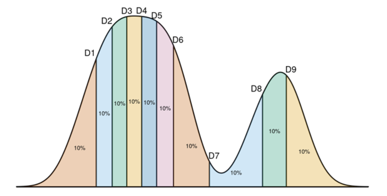
Empirical Quantile
- An empirical quantile divides 1-D data into $m$ continuous intervals with equal probability $q$.
- An empirical quantile function returns the cut-point for the interval corresponding to $q$, for qhich $(1-q)$% of the data are larger than the cut-point and $q$% are smaller than that value.

Applications of Conformal Prediction

Conformal prediction is a versatile framework with applications across domains:

Medical Triage: In critical healthcare scenarios, such as diagnosing diseases or interpreting medical images, high confidence is essential. For example, when analyzing a CT scan to determine the type of stroke a patient has, conformal prediction can ensure that the decision is statistically reliable. By setting a very low $\alpha$, the system can prioritize safety and minimize errors.
Selective Classification: Models can abstain from making a prediction when uncertainty is high. This is useful for routing difficult cases to human experts, improving overall system reliability.
Active Learning: In scenarios where labeled data is expensive to obtain, conformal prediction can identify the most uncertain samples (i.e., those with the largest prediction regions) for annotation. This approach accelerates learning while minimizing annotation costs.
Out-of-Distribution (OOD) Detection: When a test sample lies outside the distribution of the training data, conformal prediction can flag it as uncertain. This is especially useful in applications like autonomous driving or fraud detection.

Marginal vs. Conditional Coverage

Marginal Coverage: This is the standard guarantee offered by conformal prediction. It ensures that the correct prediction is included in the prediction region for at least $1-\alpha$ of all test samples, averaged across the dataset. For instance, at 90% confidence, marginal coverage ensures that at least 90% of predictions are correct on average.
Conditional Coverage: A stricter form of coverage, ensuring that predictions are correct across subgroups or classes. For example, in cancer diagnosis, we may want 99% accuracy both for patients with cancer and those without. Marginal coverage cannot guarantee fairness across such subgroups, whereas conditional coverage aims to addresss this limitation.

Recipes for Conformal Prediction

Conformal prediction recipes provide systematic steps to create prediction regions or sets for classification and regression tasks. They ensure statistical guarantees, balancing uncertainty with accuracy.

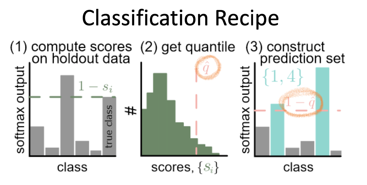
Classification Recipe

This recipe provides prediction sets for classification tasks, ensuring that the correct label is included in the set with a user-specified confidence level.

Part 1: Pre-trained Model and Calibration Data

Start with a pre-trained deep neural network (DNN) for classification.
Use a calibration set – a separate subset of data not used during training. The size of this set significantly affects the prediction quality.

Part 2: Define a Nonconformity Measure

A heuristic score function is defined based on the output of the model.
- Example: If the model uses softmax outputs, define the nonconformity score as:
  $s_i = 1-\hat{f}(X_i)_{Y_i}$
- Here, $\hat{f}(X_i)_{Y_i}$ is the softmax probability for the true class $Y_i$.
- $s_i$ measures how “wrong” the model is for a specific input $X_i$. A high score indicates high uncertainty or error.

Part 3: Compute Empirical Quantiles

Using the calibration set, calculate the quantile threshold for the desired confidence level $(1-\alpha)$:
$q=\frac{1}{n+1}(1-\alpha)$
- Here, $n$ is the size of the calibration set.
- The threshold ensures that prediction sets contain the correct class at least $1-\alpha$ of the time.

Part 4: Form Prediction Sets

For each test sample, include all classes whose nonconformity scores fall below the quantile threshold:
$C(X_{test})= \{ y:s(X_{test},y) \leq q \}$
The resulting set is guaranteed to include the correct class with high probability.

Example:

Suppose $\alpha = 0.1$, and the calibration set has 1000 samples ($n=1000$). Then $q=0.901$.
If the nonconformity scores for a test input are:
- Class A: 0.3
- Class B: 0.85
- Class C: 0.92
The prediction set includes classes A and B (since $s \leq q$)

Python Code Implementation Example:

# Step 1: Get conformal scores. n=calib_Y.shape[0]
cal_smx = model(calib_X).softmax(dim=1).numpy()
cal_scores = 1-car_smx[np.arange(n), cal_lables]

# Step 2: Get adjusted quantile
q_level = np.ceil((n+1)*(1-alpha))/n
qhat = np.quantile(cal_scores, q_level, method='higher')
val_smx = model(val_X).softmax(dim=1).numpy()
prediction_sets = val_smx >= (1-qhat) # Step 3. Form prediction sets

This algorithm takes in an input, and outputs a set of classes.
It constructs a different output set adaptively to each particular input.
Sets are larger when the image is intrinsically hard.

Regression Recipe

The regression recipe generates prediction intervals that contain the true value with high confidence.

Part 1: Pretrained Model and Calibration Data

Begin with a pre-trained regression model.
Use a clibration set (separate from training and testing data) to calculate residuals.

Part 2: Compute Residuals

For each calibration sample, compute the residual:
$r_i = \vert y_i - \hat{y_i} \vert$

$y_i$: True value , $\hat{y_i}$: Predicted value

Part 3: Determine Quantile Threshold

Compute the quantile of the residuals at the desired confidence level $(1-\alpha)$ :
$q=\text{Quantile}(r_1, r_2, \dots, r_n, \text{probability} = 1-\alpha)$
- The quantile $q$ defines the width of the prediction interval.

Part 4: Generate Prediction Intervals

For a new test input $X_{test}$, the prediction interval is:
$[ \hat{y_{\text{test}}}-q, \hat{y_{\text{test}}}+q]$
- $\hat{y_{\text{test}}}$ is the model’s prediction for prediction for $X_{\text{test}}$.
- The interval is guaranteed to contain the true value with probability $1-\alpha$
Example:
- Suppose $\alpha=0.05$ (95% confidence level).
- Calibration residuals: [1.2, 0.8, 1.5, 2.0, 1.0].
- Compute the 95th percentile quantile: $q=1.9$
- For a test prediction $\hat{y_\text{test}}=10$, the prediction interval is:
  $[10-1.9, 10+1.9] = [8.1, 11.9]$

General Recipe for Conformal Prediction

This general framework can be adapted for both classification and regression task:

Identify a Heuristic Score: Choose a measure of uncertainty (e.g., softmax output, residuals) based on the model’s predictions.
Compute Calibration Scores: Evaluate the heuristic scores for the calibration set.
Quantile Threshold: Compute the quantile $q$ based on the desired confidence level.
Prediction Regions: Use the threshold $q$ to form prediction regions or intervals for test samples.

Share on

Twitter Facebook LinkedIn

Wonha Leah Shin