
Day101 Deep Learning Lecture Review - Lecture 17 (2)
Variation of Conformal Prediction: Size of Calibration Set, Evaluation, and Group-Based & Adaptive Conformal Prediction

Calibration Set Size in Conformal Prediction
The size of the calibration set plays a crucial role in the effectiveness and reliability of conformal prediction.
- Why Calibration Set Size Matters
- Marginal Coverage: Conformal prediction guarantees correct coverage (e.g., 90% for $\alpha=0.1$) when the calibration set is exchangeable with the test set. However, the coverage relies on the randomness of the calibration set.
- Impact on Coverage: A smaller calibration set introduces more variability in the coverage guarantees, whereas a more extensive set makes the coverage guarantees more reliable.
-
Formal Guarantees
- The coverage provided by conformal prediction follows this inequality:
$1-\alpha \leq \textbf{P}(Y_\text{test}) \in C(X_{\text{test}}) \leq 1- \alpha + \frac{1}{n+1}$
-
$n$ : Size of the calibration set.
-
$\alpha$: Desired error rate (e.g., $\alpha=0.1$ for 90% confidence).
A larger $n$ reduces the additional term $\frac{1}{n+1}$, tightening the coverage bounds.
-
Choosing Calibration Set Size
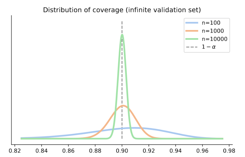
- Small Calibration Sets: Lead to high variability in coverage. For example, with $n=100$ and $\alpha=0.1$, the coverage may fluctuate between 85% and 95%.
-
Large Calibration Sets: Provide more stable coverage. For $n=1000$, the coverage typically ranges closer to the desired 90% level.
-
Example:
- Assuming 90% coverage ($\alpha = 0.1$):
- With $n=100$ : Coverage might range between 85% and 95%.
- With $n=1000$: Coverage will likely range between 88% and 92%.
- Assuming 90% coverage ($\alpha = 0.1$):
Evaluating Conformal Prediction
Evaluation of conformal prediction focuses on two key aspects:
- Correctness of Coverage: Ensuring that the statistical guarantees hold in practice.
- Adaptivity: Assessing whether the prediction regions adapt appropirately to the difficulty of inputs
-
Evaluating Coverage: Conformal prediction guarantees marginal coverage over the test set. To verify this:
-
Empirical Check:
-
Split the dataset into multiple calibration and test sets.
-
Compute the empirical coverage (fraction of correct predictions) across test samples.
-
Average the empirical coverage across multiple splits to ensure the guarantees are met.
-
The fomular for empirical coverage is below.
$C_j = \frac{1}{n_{\text{val}}} \sum_{i=1}^{n_{\text{val}}} \mathbb{1}\left(Y_i^{(\text{val})} \in C(X_i^{(\text{val})})\right)$
Where:
- $n_{\text{val}}$: Size of the validation set.
- $C(X_i^{(\text{val})})$: Prediction region for test sample $X_i^{(\text{val})}$.
-
Example:
- Perform $R$ trials with different calibration and test splits.
- Compute the mean empirical coverage across these trials to check consistency.
-
-
-
Evaluating Adaptivity:
-
Adaptivity ensures that:
- Easy Examples: Result in smaller prediction regions.
- Hard Examples: Result in larger prediction regions.
-
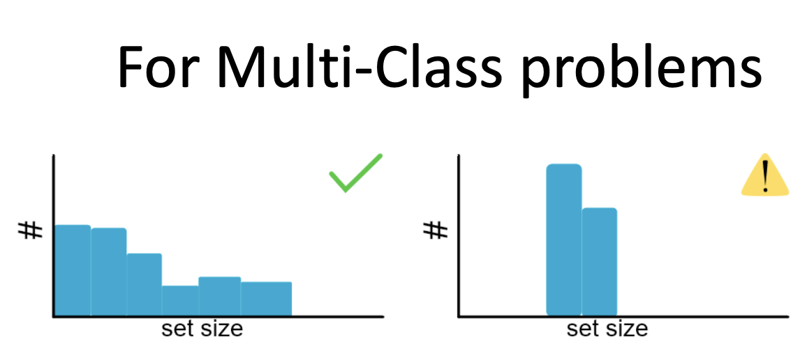
For multi-class problems, histograms of prediction set sizes can illustrate adaptivity:
- A dynamic range of set sizes indicates that the method adpats well.
- A lack of variation (e.g., all sets are large) suggests poor adaptivity.
-
-
Evaluation Metrics:
- Feature-Stratified Coverage (FSC):
- Measures conditional coverage for defined subgroups (e.g., gender or age groups).
- Evaluates the worst-case coverage across all groups.
- Size-Stratified Coverage (SSC):
- Assesses coverage across prediction sets of different sizes.
- Ensures that coverage holds even for small prediction sets.
- Class-Conditional Coverage (CCC):
- Checks coverage for individual classes in classification problems.
- Checks coverage for individual classes in classification problems.
- Feature-Stratified Coverage (FSC):
Group-Balanced Conformal Prediction
Group-balanced conformal prediction ensures that coverage guarantees are maintained for specific subgroups in the data (e.g., based on race, gender, or other attributes). This method stratifies the data into predefined groups and applies conformal prediction independently to each group.
Steps:
-
Split the data into subgroups $G_1, G_2, \dots, G_k$ where each group corresponds to a specific attribute or label.
-
For each group $G_g$, compute the conformal quantiles $\hat{q}_g$ separately using the calibration set for that group:
$\hat{q}_g = \text{Quantile}\left(\{s_i : X_i \in G_g\}, 1 - \alpha\right)$
where $s_i$ is the nonconformity score for sample $i$. -
During testing, use the group label of the test sample to apply the corresponding quantile $\hat{q}_g$:
$C(X_\text{test}) = \{y : s(X_\text{test}, y) \leq \hat{q}_g\}$
Key Essentials To Consider:
- Each group has its own prediction set, ensuring fair coverage across groups.
- Requires access to group labels for test samples, which may not always be available
Adaptive Prediction Sets (APS)
Adaptive Prediction Sets (APS) improve upon standard conformal prediction by dynamically adjusting prediction sets to provide better conditional coverage, particularly for challenging inputs or subgroups. APS addresses key issues such as overcovering easy inputs and undercovering hard inputs by leveraging adaptive score functions.
- Motivation
- In standard conformal prediction, prediction sets are determined based on a heuristic score, such as $1 - \text{softmax}$, which may not accurately reflect true uncertainty.
- APS modifies this score function to include information about both the true class and higher-scoring classes, making the prediction sets more adaptive to the difficulty of the input.
-
Score Function
-
In APS, the score function is redefined to be cumulative. Instead of focusing only on the correct class, the score includes the softmax value of the true class and all higher-ranking classes. This cumulative approach improves adaptivity.
-
The APS score function is defined as:
$ \sum_{j=1}^k \pi_j(X)$
where:
- $\pi_j(X)$: Softmax probability for the jjj-th class, sorted in descending order.
- $k$: Number of top classes contributing to the cumulative score.
-
-
Steps in APS:
-
Compute Calibration Scores:
- Use the new adaptive score function to compute scores for all calibration samples:
$s_i = \sum^{k}_{j=1} \pi_j (X_i)$
- Here, $k$ is determined dynamically based on the threshold.
-
Determine Quantile:
-
Find the conformal quantile $\hat{q}$ for the desired confidence level $(1-\alpha)$ using the calibration scores:
$\hat{q} = \text{Quantile}({s_i}, 1-\alpha)$
-
-
Form Prediction Sets:
-
For each test input $X_{\text{test}}$, add classes to the prediction set in descending order of their softmax scores until the cumulative score exceeds the quantile threshold $\hat{q}$
$C(X_\text{test}) = \{ \pi_1(X), \dots, \pi_k(X) : \sum_{j=1}^k \pi_j(X) \leq \hat{q} \}$
-
-
Advantages of APS
- Better Conditional Coverage:
- APS dynamically adjusts prediction sets to reflect the difficulty of the input.
- Hard examples result in larger sets, while easy examples result in smaller sets.
- Improved Fairness:
- APS ensures more equitable coverage across classes or subgroups by addressing biases inherent in standard methods.
- Flexibility:
- The adaptive score function can be tailored to specific datasets or models, making APS suitable for diverse applications.
Comparison with Standard Conformal Prediction
- Standard Conformal Prediction:
- Relies on fixed heuristic scores like $1 - \text{softmax}$, which can lead to overcoverage of easy inputs and undercoverage of hard ones.
- Does not explicitly address conditional coverage.
- APS:
- Introduces cumulative scores for better adaptability.
- Provides more balanced prediction sets across all inputs.
Limitations of Conformal Prediction
While conformal prediction offers formal guarantees, it is not without challenges:
- Exchangeability Assumption: The framework assumes that calibration and test sets come from the same distribution. In real-world scenarios, such as deployment in dynamic environments, this assumption may not hold. Techniques like weighted conformal prediction can address mild distribution shifts.
- Post-Hoc Nature: Conformal prediction is applied after model training and does not modify the model itself. This makes it unsuitable for applications like continual learning, where the model is continuously updated.
- Scalability: Computing prediction regions for large datasets or complex models can be computationally expensive, especially when handling high-dimensional data.
Leave a comment