Day102 Deep Learning Lecture Review - Lecture 18 (1)

📚 The Start of Recording TIL Summer ‘24 : Why Did I Start This Project? 🚀

🔔 Don't Miss: Continous Records of TIL '25 (Still On-Going!) 🌟

✨ A New Chapter in TIL '25: Reflecting, Growing, and Moving Forward 📖

Data-Centric AI: Crowdsourcing, Methods to Estimate Annotator Quality, Neural Scaling Laws, Pareto Curves and Power Law

What is Data-Centric AI?

Explanations from: MIT - Introduction to Data-Centric AI

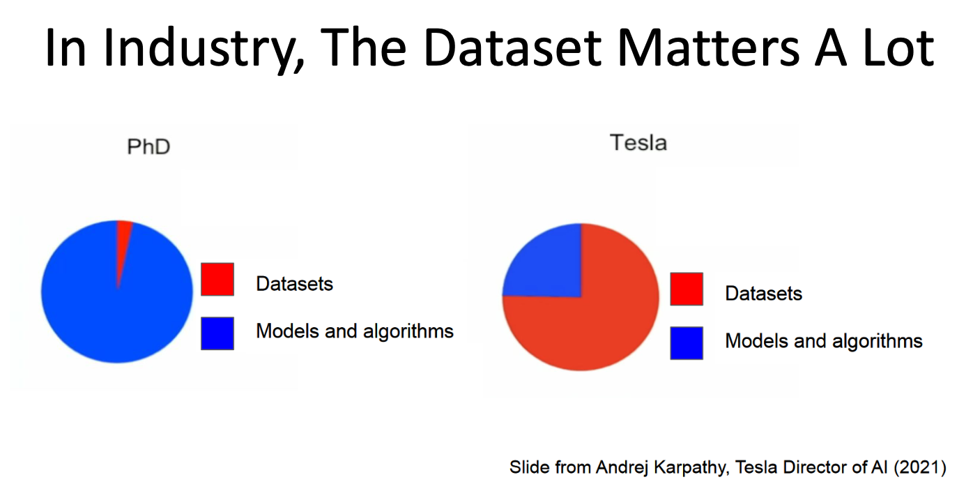
Data-centric AI focuses on systematically improving datasets to enhance model performance. Unlike Model-Centric AI, which prioritizes algorithms and architectures, Data-Centric AI shifts attention to curating, cleaning, and optimizing data.

• Data-centric AI deals with systematically engineering data to build better AI systems.
• Real-world datasets are messy, and improving the dataset can significantly improve results.
• Data-centric AI thinks about AI in terms of the data and not the specific model.
• Data-centric AI Methods
  • Outlier detection and removal
  • Detecting and correcting label errors
  • Data augmentation
  • Feature engineering and selection
  • Establishing consensus labels from crowdsourced data.
  • Active learning to select the most informative data to label next.
  • Identifying the correct data and possibly data ordering to train models.
    
    

Contrast with Model-Centric AI

• Model-centric AI works with a fixed, often curated dataset, focusing on optimizing algorithms and techniques.
• Real-world datasets are messy, and systematic dataset engineering can significantly improve skills.

Key Principles:

1. Systematic Data Engineering:
   • Addresses noisy, redundant, and unbalanced datasets to improve model accuracy.
   • Implements methods like outlier detection, label correction, and data augmentation.
2. Real-World Datasets are Messy:
   • Many datasets have labeling errors, redundant samples, or poor-quality data points. Improving these can lead to better results than scaling model size or complexity.
3. Iterative Dataset Improvements:
   • Involves ongoing refinement of datasets, which includes labeling errors correction, balancing datasets, and focusing on high-quality data.

Not Data-Centric AI:

• Doubling dataset size indiscriminately without improving data quality.
• Hand-picking data points based on subjective criteria.

Data Creation and Curation

• Data Creation is Expensive
  • Datasets may cost millions of dollars to create.
    • Many companies spend much time getting prompts and dialogues to train LLMs.
  • The COCO dataset for semantic segmentation required over 85,000 annotator hours.
    
    

• **Curating Datasets**

  • Major issues include:
    • Detecting erroneously labeled instances
    • Identifying inputs with quality problems
      • Blurry Images
    • Data deduplication
    • Removing unwanted data
      • Toxic data for LLMs
    • Ensuring no data leakage between train and data sets
      • When scraping the web, many images may be identical or modified versions of the original
        • JPEG vs. PNG
        • Crops
  • General Steps
    • Acquire large amount of data
      • Most may be unlabeled
    • Acquire labels for the data
      • Usually from a human
    • Curate the dataset to remove errors and bad dta
    • Split dataset into appropriate partitions
    • Define metrics and study design for analysis
    • Version the dataset
      
      

Crowdsourcing Labels

Crowdsourcing involves gathering labels for datasets from a distributed group of annotators, often using platforms like Amazon Mechanical Turk. This approach is especially beneficial for large-scale datasets where manual labeling of all data is impractical.

• Key Characteristics:
  • Scalable: Can label vast amounts of data quickly.
  • Low Cost: Often cheaper than relying on domain experts.
  • Diverse Perspectives: Incorporates multiple viewpoints, which can improve label quality.
    
    
• Challenges:
  1. Annotator Noise:
     • Not all annotators are equally skilled or diligent, leading to errors.
  2. Consistency:
     • Different annotators might interpret tasks differently, introducing variability.
  3. Quality Control:
     • Ensuring high-quality labels from non-expert annotators is challenging.
  4. Applications:
     • Text sentiment analysis, image recognition, medical data annotation.
       
       

Estimating Annotator Quality

To ensure reliable labels from crowdsourced data, it’s crucial to estimate the quality of each annotator. This allows identifying and weighing annotations based on annotator reliability.

Estimating Inter-Annotator Agreement

• We can quantify the confidence that a consensus label is correct via the agreement between annotations for an example:

  $\text{Agreement}_i = \frac{1}{|\mathcal{J}_i|} \sum_{j \in \mathcal{J}_i} \left[ Y_{ij} == \hat{Y}_i \right]$
  
  

• Where we are computing the average number of annotators who agreed on the label.

• We can estimate the quality of an anotator $j$ based on the fraction of their annotations that agree with the consensus label for the same example:

  $\text{Quality}_j = \frac{1}{|\mathcal{I}_{j,+}|} \sum_{i \in \mathcal{I}_{j,+}} \left[ Y_{ij} == \hat{Y}_i \right]$
  
  

  • $\text{Quality}_j$: Measures the quality of annotator $j$.

  • $\vert \mathcal{I}_{j,+} \vert $: Total number of items labeled by annotator $j$ in the subset $\mathcal{I} _{j,+}$.

  • $\sum_{i \in \mathcal{I} _{j,+}}$: Summation over all items $i$ labeled by annotator $j$ in the subset $\mathcal{I} _{j,+}$.

  • \(\left[ Y _{ij} = = \hat{Y} _i \right]\): Indicator function, which evaluates to 1 if annotator $j$’s label ($Y_{ij}$) matches the predicted/true label ($\hat{Y} _i$), and 0 otherwise.

    
    
    

Methods to Estimate Annotator Quality

• Accuracy Against Gold Standard
  • Gold Standard:
    • Provide annotators with data in which you are 100% confident of the ground truth.
    • If they poorly annotate this data, you can evaluate whether they are delivering appropriately high-quality data or merely providing you with poor results.
    • Note that for certain issues, such as semantic segmentation, there is inherent subjective variability in the annotations provided.
    • Compare annotator’s labels against a small set of verified labels.
    • $\text{Accuracy} = \frac{\text{Correct Annotations}}{\text{Total Annotations}}$

• Agreement with Other Annotators
  • Measure consistency between annnotators.
  • Common metric: Cohen’s Kappa or Fleiss’ Kappa.

• Model-Based Estimation
  • Use probabilistic models (e.g., Bayesian methods) to estimate annotator reliability based on their label history.

Problems with Majority Vote

• Resolving ties is ambiguous.
• A bad annotator and good annotator have an equal impact on estimates.
• If you cannot enumerate a specific list of classes, e.g., natural language outputs, you need many annotators to get a consensus.
  
  

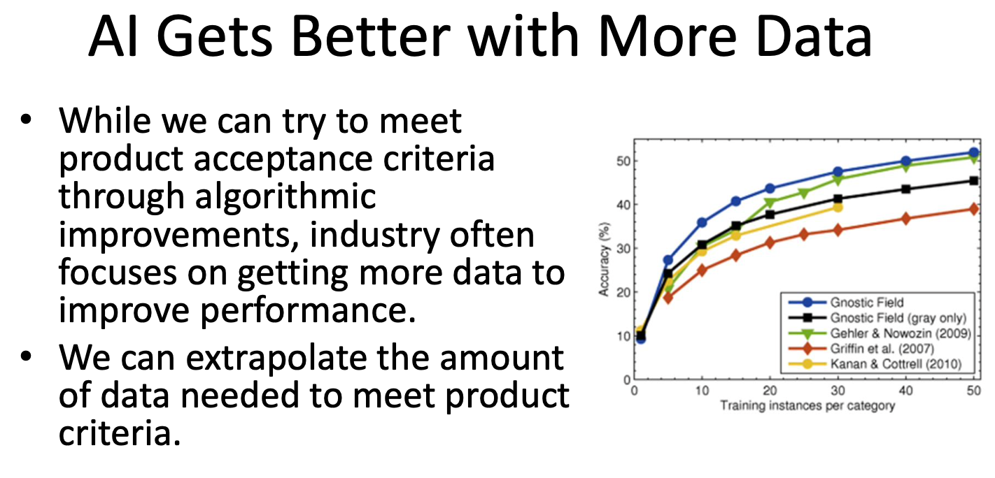
Estimating The Amount of Data We Need for Training

Determining how much data is necessary to train a machine learning model is a critical step in designing an efficient pipeline. Too little data results in underfitting, while too much data wastes resources.

• For AI products, performance needs to be greater than some threshold.

  • Often these criteria are specified by product managers.

  • Example: Cancer detection recall over 99% with less than 5% false positives.

    
    
    

Pareto Curve

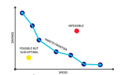
• A Pareto Curve is a graphical representation that helps illustrate trade-offs between two competing objectives, often in optimization problems or efficiency analysis. It is used to visualize the Pareto frontier, which is the set of points representing the best possible trade-offs.

Key Features:

1. Pareto Frontier:
   • The curve or boundary of the Pareto-efficient points where improving one objective leads to a degradation in the other.
   • Any point on the Pareto frontier is optimal in the sense that you cannot improve one objective without worsening the other.
2. Dominated Points:
   • Points below the Pareto curve are considered suboptimal because at least one objective can be improved without degrading the other.
3. Applications:
   • Data-Centric AI: Trade-offs between data quality and dataset size.
   • Economics: Trade-offs between cost and benefit.
   • Machine Learning: Trade-offs between model accuracy and computational cost.
     
     

Error as a Function of Training Data Follows a Power Law

In machine learning, the error (e.g., test error) of a model often decreases as the size of the training dataset increases. This relationship frequently follows a power law:

$E(n) = \frac{A}{n^b}+C$

where:

• $E(n)$: The error as a function of training data size $n$.
• $A$: A scaling constant that depends on the model and task complexity.
• $b$: The power law exponent, which indicates how quickly the error decreases as the data size grows.
• $C$: The irreducible error (Bayes error), representing the theoretical minimum error the model can achieve.
  
  

Key Features of the Power Law

• Diminishing Returns
  • As the size of training data $n$ increases, the error reduction becomes smaller.
  • For small dataset, adding more data significantly reduces error.
  • But, for larger datasets, the error reduction per additional sample diminishes.
• Scaling Laws
  • The power law demonstrates the fundamental scaling behavior of model performance with data size.
  • For complex tasks (e.g., vision, NLP), the power law exponent $b$ is typically small (e.g., $b \approx 0.5$), indicating slower improvements with data scaling.
• Universal Behavior:
  • The power law applies across many machine learning tasks and models, including surprised learning, deep learning, and even unsupervised learning tasks.
• Limitations of This Approach
  • We kept the model unchanged.
  • If the model is large, we require a minimum amount of data to derive useful points for fitting.
  • If the model is too small, the error may become irreducible because the model lacks the necessary capacity to improve with additional data.
  • Some level of error may simply be insurmountable due to the nature of the problem.