Day105 Deep Learning Lecture Review - Lecture 20 (End)

📚 The Start of Recording TIL Summer ‘24 : Why Did I Start This Project? 🚀

🔔 Don't Miss: Continous Records of TIL '25 (Still On-Going!) 🌟

✨ A New Chapter in TIL '25: Reflecting, Growing, and Moving Forward 📖

Model Drifting, Periodic Re-Training, Detecting Model Drift, Continual Learning (Pre-Trained Model, NCC), and Real-Time Machine Learning

Model Drift and Monitoring in AI Systems

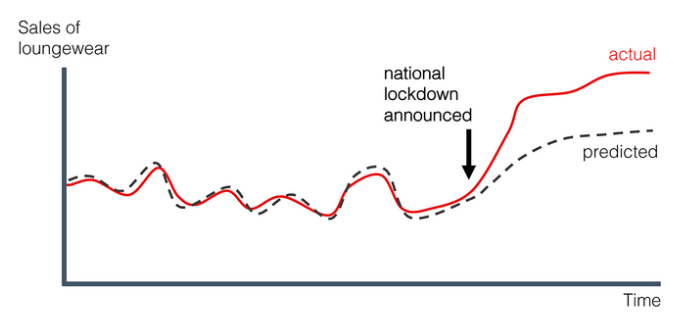
Model Drift refers to the phenomenon where an AI model’s performance degrades over time due to changes in the environment or data. This can result in unreliable predictions, potentially causing errors in applications like healthcare, finance, or autonomous systems.

As AI systems increasingly drive critical applications, guaranteeing consistent performance over time becomes a significant challenge. This is where model drift and monitoring are essential.

• Example cases

  • Model Predicted vs. Actual Loungeware Forecasting Due to Covid
    
    
    
    

  • Loan approval models trained on data from 5-6 years back.

    • Differences in financial levels of today’s customers.
    • Market/stock predictions after a natural disaster.
      
      

• Implications of Model Drift

  • Reduced Model Performance: A model that was initially accurate may become increasingly unreliable over time
  • Costly Errors: Model drift can lead to potentially life-threatening situations in safety-critical applications, such as autonomous vehicles or medical diagnoses.
  • Model Degradation: Addressing this issue may require frequent retraining, which can be resource-intensive.
    
    

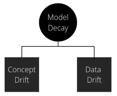
Main Causes of Model Drift (Decay)

• Model decay occurs due to changes in the statistical properties of the data between deployment and training.

• Two primary types of changes to the data.
  

  
  
  

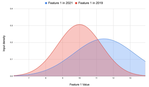
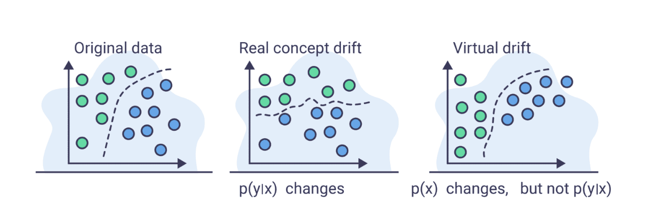
  1. Feature Drift ($P(X)$):

     • Changes occur in the input variables without altering their relationship to the target variable.

     • Example: A sensor’s calibration changes the range of temperature readings.
       Image Source: What is Data Drift and How to Detect it in Computer Vision?
       
       

     • Typical causes of Feature Drift

       • Non-stationary environment: The training environment differs from the test environment due to temporal or spatial changes.
       • Sample selection bias: Training data does not align with the deployment data.
         • We need evaluation data that matches the real-world distribution to measure the model’s efficiency.
           
           

  2. Concept Drift ($P(Y \vert X)$):

     • The relationship between the inputs (X) and target variable (Y) changes over time.

     • Example: Customer preferences shift, leading to different product purchages.

     • Three main categories
       
       

       
       
       
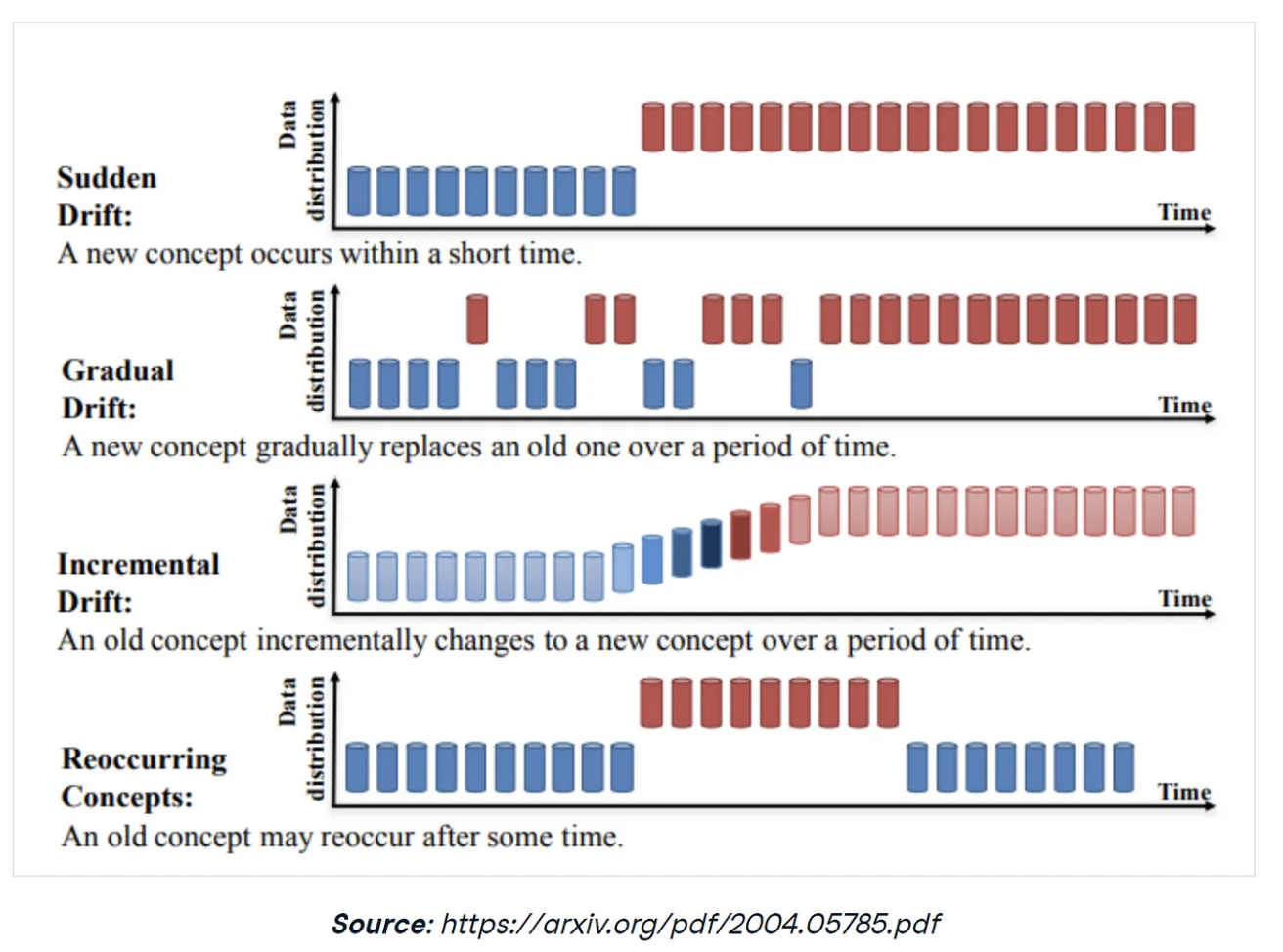
       • Sudden Drifts: Abrupt changes in the data distribution
       • Gradual Drifts: Slow and steady changes in the data distribution.
       • Seasonal Drifts: Data distribution varies periodically, often based on time-based patterns.
         • Annual treands, holidays, etc.
           
           

Main Causes of Model Drift

1. Evolving Data:
   • Real-world data distributions are dynamic and rarely remain static over time.
   • Example: COVID-19 altered consumer behaviors worldwide.
2. Data Collection Mechanisms:
   • Updates in how data is collected (e.g., new sensors or methods) can introduce discrepancies.
3. Feedback Loops:
   • Model predictions influence future data, causing the distribution to shift.
   • Example: Recommender systems streering users toward specific content.
     
     

• Impact of Model Drift
  • Degraded model accuracy and reliability
  • Increased errors in critical applications
  • Resource-intensive retraining processes
    
    

Virtual Drift and Prior Probability Shift

1. Virtual Drift

   Virtual drift is a feature shift that doesn’t affect the decisions/predictions made by the model.

   • Refers to apparent changes in model performance that arise due to external changes, not because of actual data or concept drift.
     
     Image Source: Aporia / Concept Drift in Machine Learning
     
     
     
   • Example: A shift in evaluation metrics or user behavior that affects how model performance is perceived.
     
     

2. Prior Probability Shift

   • Occurs when the base rate of target classes changes in the dataset.
   • Example: Seasonal changes in sales data where certain products are purchased more frequently during holidays.

• Such shifts might not always require model retraining; adjustments to downstream decision-making processes may suffice.
  
  

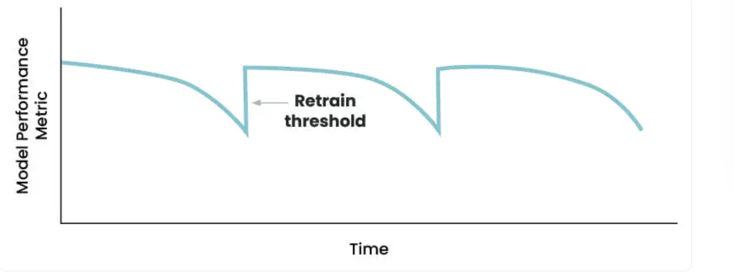
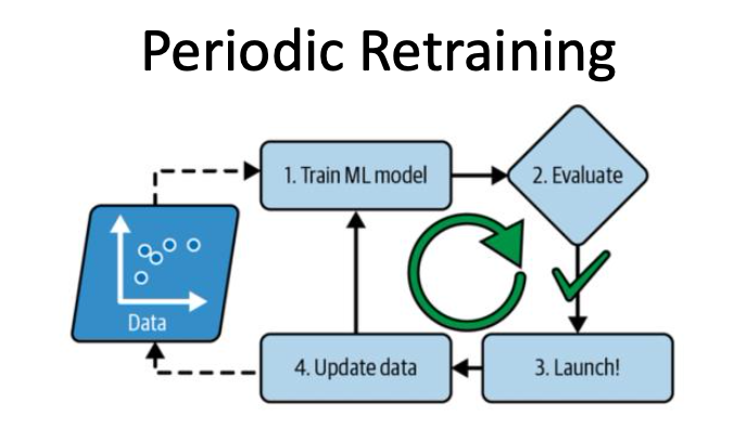
Periodic Retraining for Drift

• Periodic Retraining is common in industry.

  • Models are often retrained to address model drift.
    

    Image Source: phData: When to Retrain Machine Learning Models?

    
    
    
    
    

Retraining Techniques

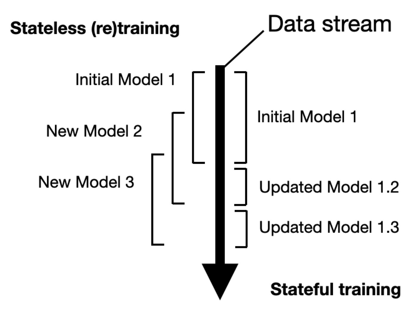
1. Stateless vs. Stateful Retraining

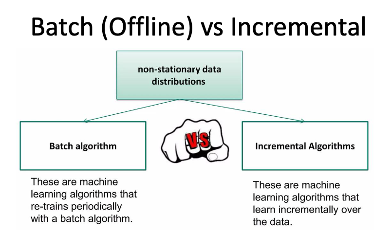
   • Stateless Retraining

     • Retrains the model from scratch using new data.
     • Often involves a fixed-sized sliding window over recent data.
     • Suitable for systems with limited historical dependencies
     • Often called “batch learning”

   • Stateful Retraining

     • Incrementally updates the existing model.
     • Utilizes methods from continual learning to retrain past knowledge.
     • Reduces computational costs for systems requiring frequent updates.
       
       

     • Image Source: Sebastian Raschka - Machine Learning FAQ
       

       
       
       
     • Differences
       • Stateless (Re)training : Stateless training is a traditional method where an initial model is trained on a specific set of data. Once this model is created, it can be retrained regularly as new data comes in. This approach, known as stateless retraining, does not keep any previous state information.
       • Stateful Training : In contrast, stateful training takes a different approach. The model starts by being trained on a batch of data, forming a base level of knowledge. Instead of fully retraining, the model is updated as new data arrives. This allows the model to adjust over time, making it better at responding to changes while maintaining what it has already learned.
         
         
2. Grubhub Case Study
   • Daily Retraining
     • Model retrained on 30 days of data daily, costing approximately $1,080 per month on AWS.
     • Achieved a 20% increase in Purchase Through Rate (PTR) compared to weekly retraining.
   • Online Updates
     • Incremental updates reduced costs by 45x compared to stateless methods.
       
       

Online Updates and Recommendations

1. Challenges with Online Updates
   • Can lead to catastophic forgetting if distribution shifts are abrupt.
   • Requires careful tuning to balance learning new data while retaining past knowledge.
2. Questions to Address Before Retraining
   • Should all data or a subset be used?
   • What retraining method (stateful/stateless) is best for the scenario
3. Important Considerations
   • Retraining alone may not address all issues; hyperparameters and model architecture might need adjustment.
   • Stateful retraining demands a deep understanding of changes in the data.
     
     

Detecting Model Drift

• The importance of monitoring
  • Model drift detection is a critical aspect of MLOps, ensuring that machine learning systems remain reliable in production environments.
  • Drift can lead to significant performance degradation if not identified and addressed promptly.
• Key Types of Drift to Monitor
  1. Feature Drift: Changes in the input data distribution $P(X)$.
  2. Concept Drift: Changes in the relationship between features and target labels $P(Y \vert X)$.
  3. Model Shift: Degradation of the model’s decision boundary over time.
     
     

Techniques for Drift Detection

• Statistical Tests for Distribution Similarity
  1. Kolmogorov-Smirnov Test (K-S Test)
     • A nonparametric test comparing two distributions (training data vs. new data).
     • Works only for univariate data and is highly sensitive to deviations.
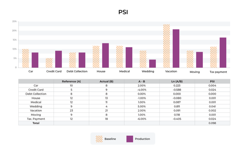
  2. Population Stability Index (PSI)
     • Measures the similarity between two distributions using a scaled version of Jensen-Shannon divergence.
     • Commonly used in finance to track changes in customer or trasaction data.
       
       
       
  3. Maximum Mean Discrepancy (MMD)
     • Compares the distributions of embeddings in high-dimensional space.
     • Provides a scalar score for the similarity between two multivariate dataests.
       
       
• Model-Based Drift Detection
  • Binary Classification Approach
    • Train a classifier to distinguish between the original training data and the new data.
    • A high classification accuracy indicstes a significant drift.
      
      

Performance Monitoring

• Golden Dataset Validation
  • A curated golden dataset with human-labled eaxmples is used for continous vlidation.
  • The model’s predictions are compared against this dataset to ensure consistency.
• Monitoring Metrics
  • Precision, Recall, F1-Score, and Area Under the ROC Curve (AUC-ROC).
  • For regression models, metrics like Mean Absolute Error (MAE) and Root Mean Square Error (RMSE) are monitored.
    
    

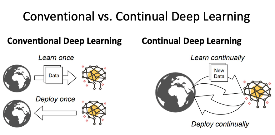
Incremental Learning

Incremental learning involves updating a machine learning model continuously as new data arrives, without retraining the model from scratch.

• Limitation of traditional ML
  • We can't keep models updated with new information without periodic re-training.
  • Updating models requires retraining from scratch is not efficient.
  • Poorly suited for personalization of models.
    
    

• Algorithms are categorized as follows:
  • Incremental Learning, Lifelong Learning, Real-Time ML, Continual Learning, Online Learning, Online Continual Learning, Streaming Learning…
• Advantages
  • Reduces computational costs compared to batch retraining.
  • Enables real-time adaptation in dynamic environment.
  • Ideal for personalization, such as recommendation system.
• Challenges
  • Catastrophic Forgetting: The tendency of neural networks to forget previously learned information when trained on new data.
  • Distribution Shift: Abrupt changes in data distribution make incremental updates unreliable without proper mitigation.
    
    
• Types of Incremental Learning

1. Online Learning: Continous updates using incoming data streams.
2. Continual Learning: Balances new learning with retaining past knowledge.
3. Streaming Learning: Focuses on efficiently learning from data presented sequentially.
   
   

Real-Time Machine Learning

Real-time ML integrates live data streams into training process, updating the model while ensuring timely inference.

• Primary Use Cases
  • Fraud Detection: Adapt to new fraud patterns as they emerge.
  • Recommender systmes: Adjust recommendations based on user activity.
  • Autonomous Vehicles: Respond to dynamic environmental changes.
• Implementation
  • Frequent incremental updates to models.
  • Trade-offs between update frequency and computational overhead.
  • Effective for scenarios where prediction latency is critical.
    
    

Continual Learning

• Online Learning Can Work If Shifts Are Slow
  • Online updates can be effective, but only if shifts are gradual.
  • Sudden shifts can lead to significant forgetting with backpropagation.
  • If new data isn’t arriving often, then each update may not sufficiently impact learning.
    
    
• Naive Fine-Tuning on New Data Doesn’t Work
  • Online updates—merely updating the network with new data—are ineffective with conventional methods due to catastrophic forgetting that occurs with gradient descent when there is a distribution shift.
  • The network forgets previously learned information and only acquires new data.
    • The greater the distribution shift, the more catastrophic forgetting occurs.
  • This problem is especially severe with incremental class learning.
    
    
• Key characteristics
  • Continual learning methods are designed to compensate for **significant** levels of distribution shift to prevent catastrophic failures.
  • Unfortunately, many only work for specific distributions.
    • The exceptions, in general, are:
      • Replay-based models
      • Methods that do not learn hidden variables representations.
  • Handles both gradual and abrupt distribution shifts.
    • Many real-world applications involve slow distribution shifts, rather than the abrupt distribution shift used in continual learning experiments.
    • Almost all systems are designed only for streams with strong shifts and no revisiting in continual learning.
      
      

Approaches to Mitigation

1. Replay-Based Methods:
   • Store past data in a buffer for re-use during training.
   • Balance learning from old and new data.
   • Example: Grubhub uses replay buffers to mitigate preference shifts in food recommendations.
2. Pre-Trained Models:
   • Use strong embeddings from pre-trained models (e.g., BERT or CLIP) to avoid relearning foundational patterns.
3. Regualarization Techniques
   • Add penalties to the loss function to limit changes in previously learned parameters.
4. Sparse Representation
   • Employ sparse architectures to minimize overlap in learned features.
     
     

Continual Learning for Real-World Applications

• Production AI Systems
  • Large-scale systems, such as search engines, frequently retrain models using batch data.
  • Incremental learning reduce costs and greenhouse emissions by optimizing retraining cycles.
• Emerging Trends
  1. Low-Shot Learning
     • Learning with minimal labeled data.
     • Critical for personalization and edge AI systems.
  2. Efficient Updates
     • Strategies to reduce computational resources during updates while maintaining model accuracy.
       
       

Primary Techniques in Continual Learning

1. Using Pre-trained Model
   • Why Pre-Trained Model?
     • Catastrophic Forgetting occurs when new training disrupts the hidden representations in earlier layers of a neural network.
     • Strong pre-trained backbones (e.g., ResNet, BERT) provide robust features that mitigate this disruption.
2. Approaches
   • Nearest Neightbor
     • Stores embeddings from pre=trained models.
     • Predictions are based on the nearest stored embedding.
   • Nearest Centroid Classifier (NCC)
     • Maintains a running average for each class.
     • Predictions are made by finding the closest centroid.
3. Advantages
   • Eliminates the need for backpropagation for learning.
   • More computationally efficient than full retraining.
     
     

Nearest Centorid Classifier

NCC computes the average feature representation (centroid) for each class during training. During inference, it assigns labels based on the nearest centroid.

• Advantages
  • Simple and effective for incremental updates.
  • Can use exponential moving averages to adapt to gradual shifts in data.
• Limitations
  • Treats all feature dimensions equally, which may not always be optional.
    
    

Streaming Linear Discriminant Analysis (SLDA)

SLDA extends NCC by considering covariance between features. It updates a shared covariance matrix among classes for better decision boundaries.

• Applications
  • Achieved the highest accuracy among streaming methods with minimal computational resources.
  • Requires only 0.001 GB beyond the CNN and completes training 100x faster than traditional models.
    
    
    

This is the end of the lecture.