Day11 ML Review - Gradient Descent (1)

📚 The Start of Recording TIL Summer ‘24 : Why Did I Start This Project? 🚀

🔔 Don't Miss: Continous Records of TIL '25 (Still On-Going!) 🌟

✨ A New Chapter in TIL '25: Reflecting, Growing, and Moving Forward 📖

Basic Concepts, Steps, and Key Consideration

Gradient Descent is a fundamental optimization algorithm for finding a local minimum of a differentiable function. In machine learning, gradient descent is used to find the values of a function’s parameters (coefficients) that minimize a cost function as far as possible.

“A gradient measures how much the output of a function changes if you change the inputs a little bit.”

Basic Concept

The core idea behind gradient descent is to iteratively adjust the parameters of a model to minimize the target function. The algorithm uses the function’s gradient (the vector of partial derivatives) at the current point to determine the direction in which the function decreases most rapidly. The parameters are then updated in the gradient’s opposite direction, moving towards the function’s minimum.

Steps in Gradient Descent

1. Initialization: Start with initial guesses for the parameters. This can be random or based on some heuristic.

2. Compute Gradient: Calculate the cost function’s gradient with respect to each parameter. The gradient indicates the direction of the steepest ascent in the cost function.

3. Update Parameters: Adjust the parameters in the opposite direction of the gradient. This is done using the formula:

   $$ \theta = \theta - \alpha \cdot \nabla_\theta J(\theta) $$

   Where:

   • $\theta$ represents the parameters.

   • $\alpha$ is the learning rate, a tuning parameter that determines the step size during the update.

   • $\nabla_\theta J(\theta)$ is the gradient of the cost function at the current parameters.

     
     

4. Repeat: Repeat the process until the cost function converges to a minimum or until a maximum number of iterations is reached.

Key Considerations

• Learning Rate $\alpha$: The choice of learning rate is crucial. Too small $\alpha$ rate makes the convergence slow, while too large can lead to overshooting the minimum or even divergence.
• Convergence: Determining when the algorithm has converged to a minimum can be non-trivial. Common criteria include setting a maximum number of iterations or stopping when the change in cost function between iterations is below a certain threshold.
• Feature Scaling: Gradient descent can converge much faster if all features are on a similar scale and close to normally distributed. Techniques like feature normalization or standardization are often used before model training.

Explanation from https://builtin.com/data-science/gradient-descent

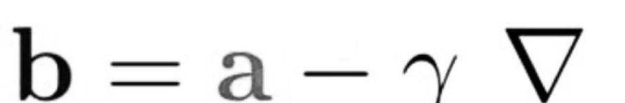
The equation below describes what the gradient descent algorithm does: b is the next position of our climber, while a represents his current position. The minus sign refers to the minimization part of the gradient descent algorithm. The gamma in the middle is a waiting factor, and the gradient term ( Δf(a) ) is simply the direction of the steepest descent.

Imagine you have a machine learning problem and want to train your algorithm with gradient descent to minimize your cost-function J(w, b) and reach its local minimum by tweaking its parameters (w and b). The image below shows the horizontal axes representing the parameters (w and b), while the cost function J(w, b) is represented on the vertical axes. Gradient descent is a convex function.

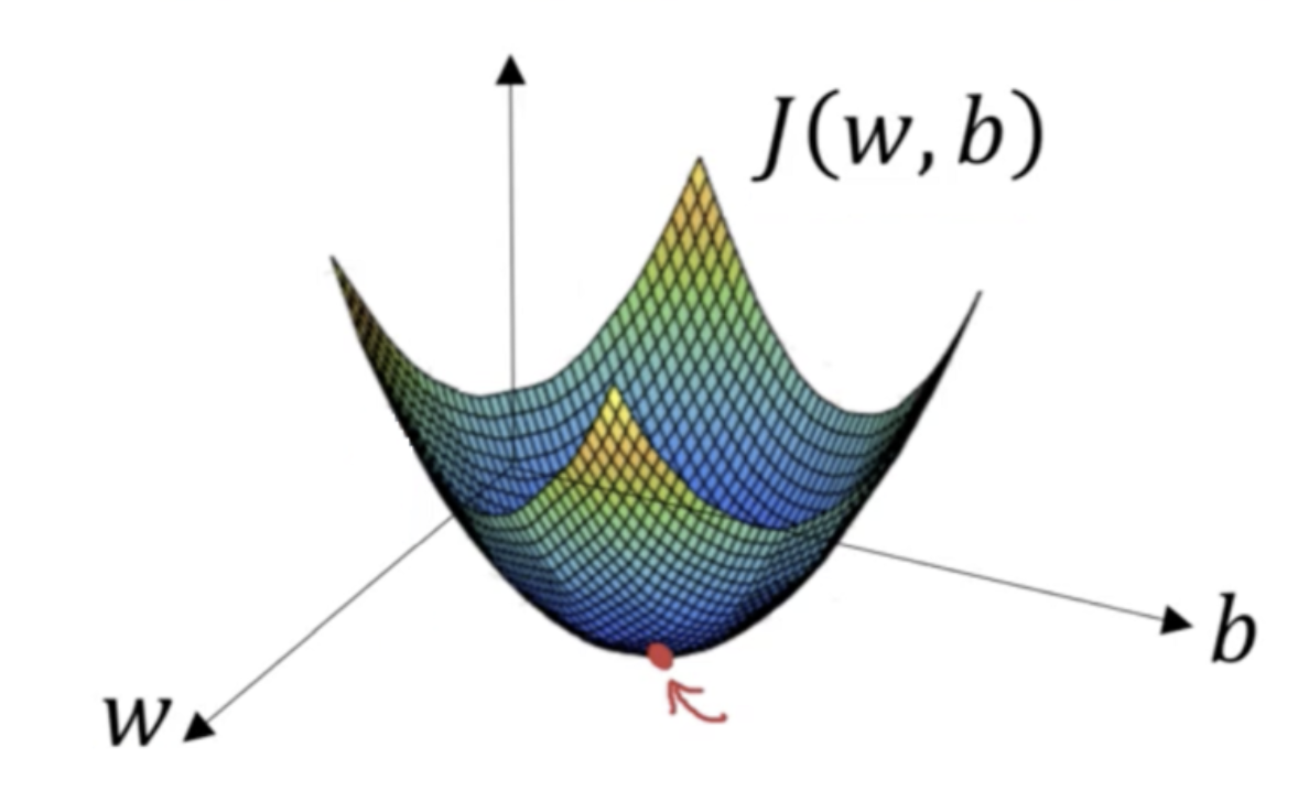
We know we want to find the values of w and b that correspond to the minimum of the cost function (marked with the red arrow). To find the right values, we initialize w and b with random numbers. Gradient descent then starts at that point (somewhere around the top of our illustration), and it takes one step after another in the steepest downside direction (i.e., from the top to the bottom of the illustration) until it reaches the point where the cost function is as small as possible.

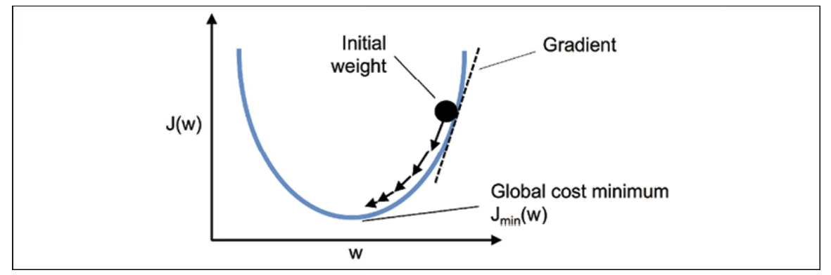
Gradient Descent Learning Rate

The learning rate determines how many steps gradient descent takes in the direction of the local minimum, which determines how fast or slow we will move towards the optimal weights. We must set the learning rate to an appropriate value for the gradient descent algorithm to reach the local minimum.

Let’s assume we have data and want to fit a regression line.

• We need to set up a line y = mx + b
• So, we need to find the optimal b and the optimal m
• Standard approach:
  • Define an error function that measures how “good” a given line is
  • This function will take in potential values for (m, b) pair and find the lowest SSE by calculating it
  • If we minimize the SSE, we will get the best line for our data

Let’s say we have a simple linear regression: y_pred = mX + b

• Step 1: Initialize the weights (intercept and slope) with random values and calculate SSE
• Step 2: Calculate the gradient (or the change) at the initial values for intercept and slope
• Step 3: Change the initial values of intercept and slope by subtracting the product of the learning rate and gradient for each parameter and adjust the weights with the gradients to reach the optimal values (goal: minimizing SSE)
• Step 4: Use the new weights for prediction and to calculate the new SSE. If it exists, compare the new SSE to the previous SSE
• Step 5: Repeat Step 2 and Step 3 until further adjustments to weights do not significantly reduce the error

The core idea behind gradient descent is to iteratively adjust a model’s parameters (or weights) to minimize a cost function. The direction and magnitude of the adjustment are determined by the gradient (or the first derivative) of the cost function at the current point. By moving in the direction opposite to the gradient (the direction of the steepest ascent), you can reach the local minimum of the function.