Day13 ML Review - Gradient Descent (3)

📚 The Start of Recording TIL Summer ‘24 : Why Did I Start This Project? 🚀

🔔 Don't Miss: Continous Records of TIL '25 (Still On-Going!) 🌟

✨ A New Chapter in TIL '25: Reflecting, Growing, and Moving Forward 📖

Summarization and Types

from: https://www.ibm.com/topics/gradient-descent

Gradient descent is an optimization algorithm commonly used to train machine learning models and neural networks. It trains machine learning models by minimizing errors between predicted and actual results.

Training data helps these models learn over time, and the cost function within gradient descent specifically acts as a barometer, gauging its accuracy with each iteration of parameter updates. Until the function is close to or equal to zero, the model will continue to adjust its parameters to yield the smallest possible error. Once machine learning models are optimized for accuracy, they can be powerful tools for artificial intelligence (AI) and computer science applications.

How Does Gradient Descent Work?

It may help to review some concepts from linear regression before we jump into the gradient descent. We may recall the following formula for the slope of a line, which is $y = mx + b$, where $m$ represents the slope and $b$ is the intercept of the $y$ -axis.

We may also recall plotting a scatterplot in statistics and finding the line of best fit, which required calculating the error between the actual output and the predicted output ($y-hat$) using the mean squared error formula. The gradient descent algorithm behaves similarly but is based on a convex function.

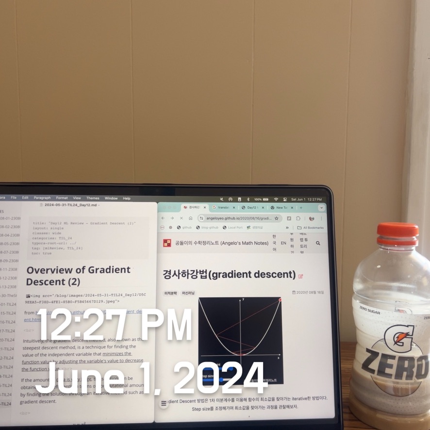
The starting point is just an arbitrary point for us to evaluate the performance. From that starting point, we will find the derivative (or slope), and from there, we can use a tangent line to observe the steepness of the slope. The slope will inform the updates to the parameters - i.e., the weights and bias. The slope at the starting point will be steeper, but as new parameters are generated, the steepness should gradually reduce until it reaches the lowest point on the curve , known as the point of convergence.

Similar to finding the line of best fit in linear regression, the goal of gradient descent is to minimize the cost function or the error between predicted and actual $y$.

To do this, two data points are required—a direction and a learning rate. These factors determine the partial derivative calculations of future iterations, allowing them to gradually arrive at the local or global minimum (i.e., the point of convergence).

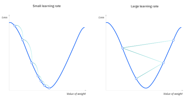
• Learning Rate (also called step size or the alpha) is the size of the steps taken to reach the minimum. This is typically a small value, and it is evaluated and updated based on the behavior of the cost function. High learning rates result in larger steps but risks overshooting the minimum. Conversely, a low learning rate has small step sizes. While it has the advantage of more precision, the number of iterations compromises overall efficiency as this takes more time and computations to reach the minimum.
• The cost (or loss) function measures the difference, or error, between actual $y$ and predicted $y$​​ at its current position. This improves the machine learning model’s efficacy by providing feedback to the model to adjust the parameters to minimize the error and find the local or global minimum. It continuously iterates, moving along the direction of the steepest descent (or the negative gradient) until the cost function is close to or at zero. At this point, the model will stop learning. Additionally, while the terms cost function and loss function are considered synonymous, there is a slight difference between them. It’s worth noting that a loss function refers to the error of one training example, while a cost function calculates the average error across an entire training set.

Types of gradient descent

There are three types of gradient descent learning algorithms: batch gradient descent, stochastic gradient descent, and mini-batch gradient descent.

Batch Gradient Descent

Batch gradient descent sums the error for each point in a training set, updating the model only after all training examples have been evaluated. This process is referred to as a training epoch.

While this batching provides computation efficiency, it can still have a long processing time for large training datasets as it still needs to store all of the data in memory. Batch gradient descent also usually produces a stable error gradient and convergence, but sometimes, that convergence point isn’t ideal, finding the local minimum rather than the global one.

Stochastic Gradient Descent

Stochastic gradient descent (SGD) runs a training epoch for each example within the dataset and updates each training example's parameters one at a time. Since you only need one training example, they are easier to store in memory. While these frequent updates can offer more detail and speed, they can result in losses in computational efficiency when compared to batch gradient descent. Its frequent updates can result in noisy gradients, but this can also be useful in escaping the local minimum and finding the global one.

Mini-batch Gradient Descent

Mini-batch gradient descent combines concepts from batch and stochastic gradient descent. It splits the training dataset into small batch sizes and performs updates on each of those batches. This approach balances the computational efficiency of batch gradient and the speed of stochastic gradient descent.

Challenges with Gradient Descent

While gradient descent is the most common approach for optimization problems, it comes with its own challenges. Some of them include:

Local Minima and Saddle Points

For convex problems, gradient descent can find the global minimum with ease, but as nonconvex problems emerge, gradient descent can struggle to find the global minimum, where the model achieves the best results.

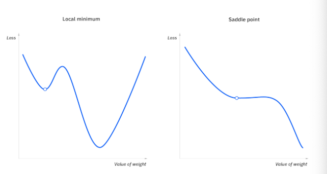
Recall that when the slope of the cost function is at or close to zero, the model stops learning. A few scenarios beyond the global minimum can also yield this slope: local minima and saddle points. Local minima mimic the shape of a global minimum, where the slope of the cost function increases on either side of the current point. However, with saddle points, the negative gradient only exists on one side of the point, reaching a local maximum on one side and a local minimum on the other. Its name is inspired by that of a horse’s saddle.

Noisy gradients can help the gradient escape local minimums and saddle points.

Vanishing and Exploding Gradients

In deeper neural networks, particularly recurrent neural networks, we can also encounter two other problems when the model is trained with gradient descent and backpropagation.

• Vanishing Gradients: occur when the gradient is too small. As we move backward during backpropagation, the gradient continues to become smaller, causing the earlier layers in the network to learn more slowly than the later layers. When this happens, the weight parameters update until they become insignificant—i.e., 0—resulting in an algorithm that is no longer learning.
• Exploding Gradients: This happens when the gradient is too large, creating an unstable model. In this case, the model weights will grow too large and eventually be represented as NaN. One solution to this issue is to leverage a dimensionality reduction technique, which can help minimize complexity within the model.