Day17 ML Review - Regularization

📚 The Start of Recording TIL Summer ‘24 : Why Did I Start This Project? 🚀

🔔 Don't Miss: Continous Records of TIL '25 (Still On-Going!) 🌟

✨ A New Chapter in TIL '25: Reflecting, Growing, and Moving Forward 📖

Concepts, Types of Regularization, and How It Works

Regularization in machine learning is a technique used to prevent overfitting. Overfitting happens when a model works well with the training data but performs poorly with new, unseen data. This usually occurs in complex models with too many parameters relative to the number of observations. Regularization solves this problem by imposing a penalty on the size of the coefficients. It prevents the model from learning the training data too well and reducing the loss too quickly by adding a penalty term. This helps to avoid overfitting by slowing down the reduction of loss. Regularization is any modification to a learning algorithm intended to reduce its generalization error but not its training error.

Explanation from: https://deepdata.tistory.com/88

Underfitting & Overfitting

• Underfitting: Not capturing enough patterns in the data. Perform poorly on both train & test datasets.

• Overfitting: occurs when a model captures both the patterns and noise in the training data, which leads to poor performance on unseen data. In simpler terms, noise refers to the presence of irrelevant data. In this context, the noise exists only in the training data. When a model trained with this noise encounters new test data, its performance suffers because the noise present in the training data does not exist in the test data. Various regularization techniques have been proposed to address overfitting. These techniques involve making minor adjustments to the model’s learning algorithm to improve its generalization of new data.

Types of Regularization

L1 Regularization (Lasso Regression)

• Adds a penalty equivalent to the absolute value of the magnitude of coefficients.
• Formula: $\lambda \sum |w_i|$ where $\lambda$ is the regularization strength and $w_i$​ are the model coefficients.
• This can result in some coefficients being set to zero, leading to feature selection. L1 regularization helps reduce overfitting and select features by removing uninformative features from the model. It is used when we want to lessen the number of features in a model, especially if we think many features are not relevant or unnecessary.
  
  

L2 Regularization (Ridge Regression)

• Adds a penalty equivalent to the square of the magnitude of coefficients.
• Formula: $ \lambda \sum w_i^2 $
• All coefficients are shrunk by the same factor (none are zeroed out completely). This is used when we suspect many features influence the outcome, but their effect sizes are small or moderate.
• It handles models affected by multicollinearity better (where independent variables are highly correlated).
  
  
  
  

Explanation & Image from Sebastian Raschka and Vahid Mirjalili, "Python Machine Learning: Machine Learning and Deep Learning with Python, scikit-learn, and TensorFlow 2," 3rd Edition, Packt Publishing, 2019.

How Regularization Works

In machine learning, regularization is a technique that entails adding a penalty term to the loss function to prevent overfitting. The loss function, which measures the deviation between predicted and actual values, comprises two components: the prediction error term and the regularization term. The aim is to discover the most suitable combination of weight coefficients that lowers the cost function for the training dataset. The accompanying figure illustrates this process to represent the concept visually.

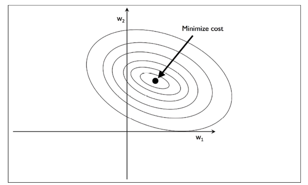
Cost Function

By increasing the regularization strength with the regularization parameter $\lambda$, we shrink the weights toward zero and reduce the reliance of our model on the training data.

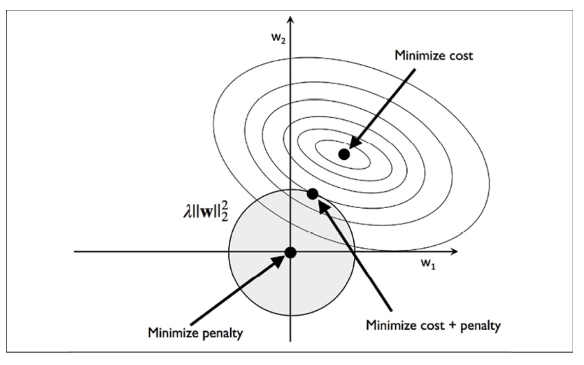
L2 Regularization

The shaded ball in the diagram symbolizes the quadratic L2 regularization term. This implies that our weight coefficients are bounded by our regularization budget, and their combination must remain within the shaded region. Despite this limitation, our objective is to minimize the cost function.

Due to the penalty constraint, our primary aim is to identify the point at which the L2 ball intersects with the contours of the unpenalized cost function. As the regularization parameter increases, the penalized cost escalates more rapidly, resulting in a narrower L2 ball.

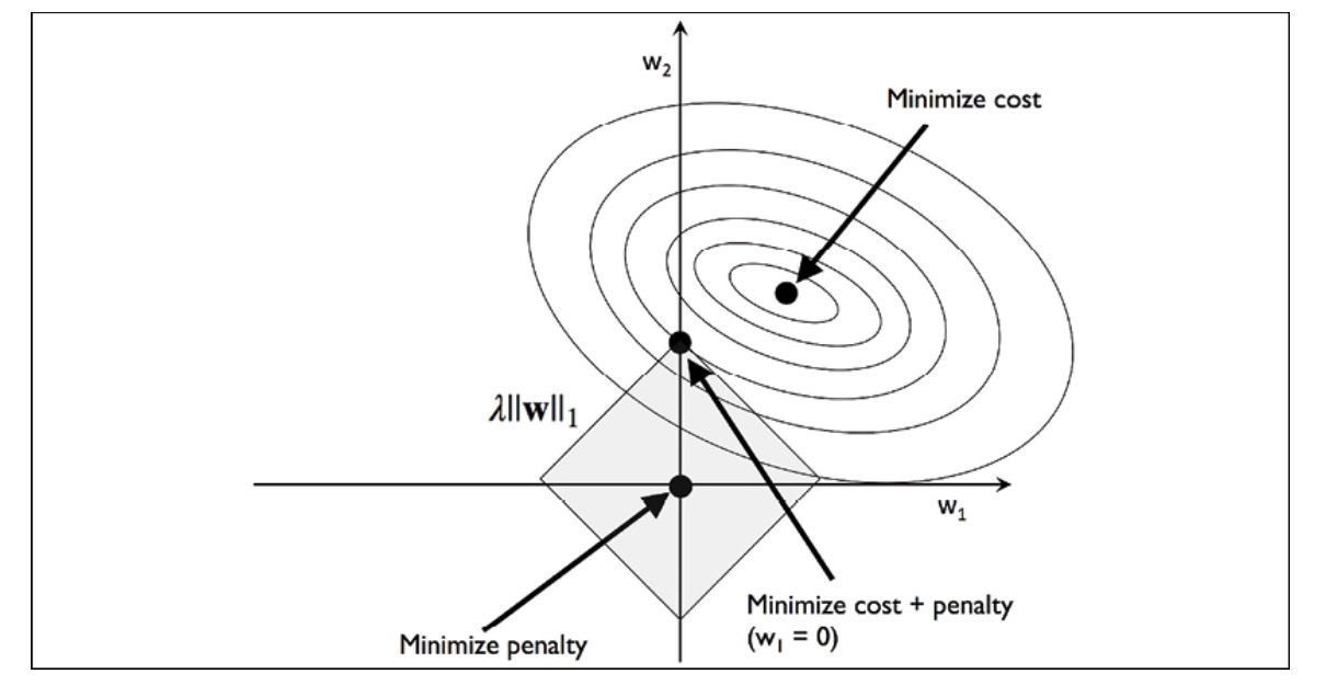
L1 Regularization

In the context of L1 regularization, the penalty is determined by the sum of the absolute weight coefficients, as opposed to the quadratic nature of the L2 penalty. This concept can be understood as a budget in the shape of a diamond. When examining the cost function contour, it becomes clear that it intersects with the L1 diamond at a specific point. Given the sharp contours of an L1 regularized system, the optimal intersection between the ellipses of the cost function and the boundary of the L1 diamond is likely to be situated on the axes. This encourages sparsity within the model.

Including the regularization term controls the complexity of the model, ensuring that the model coefficients do not fit the noise in the training data too closely. This is achieved by:

• Increasing $\lambda$: Leads to smaller coefficients, which can reduce overfitting but increase underfitting.
• Decreasing $\lambda$: Leads to larger coefficients, allowing the model to fit the data better but risking overfitting.
  
  

Practical Implications:

In practice, the choice of regularization technique and the tuning of the regularization parameter($\lambda$) are critical. These are often selected through cross-validation, where different values are tried, and the one that performs best on a hold-out set is chosen.

Regularization is a foundational concept in machine learning, applicable across various models, including linear/logistic regression, neural networks, and more, helping improve model generalization.

For regularized models in scikit-learn that support L1 regularization, we can set the penalty parameter to L1 to obtain a sparse solution.

from sklearn.linear_model import LogisticRegression
LogisticRegression(penalty='l1', solver='liblinear', multi_class='ovr')

Goal and Benefits of Regularization

• Prevent Overfitting
  • Regularization reduces the model’s complexity by constraining its coefficients, discouraging overly complex models that fit the noise in the training data.
• Improve Model Generalization
  • Simplified models perform better on new, unseen data because they capture the underlying trends rather than the specifics of the training set.
• Handle High Dimensionality
  • Regularization is particularly useful when the number of features (variables) exceeds the number of observations, making models unstable or prone to overfitting.
• Feature Selection:
  • Some features can be eliminated from the model, especially with L1 regularization, helping identify the most important features for predicting the target variable.

Side Note: High Dimensionality Issues

Several challenges arise in scenarios with more features (variables) than data points (observations).

• Overfitting: occurs when a model quickly learns the noise in the training data rather than the underlying pattern. This results in an outstanding performance on the training data, but the generalization needs to be improved to new, unseen data.
• Computational Complexity: more features increase the computational burden, as more parameters need to be estimated.
• Multicollinearity: high dimensionality often brings about multicollinearity, where some variables are highly correlated. This redundancy can destabilize the model, leading to unreliable and highly variable estimates of regression coefficients.