Day20 Probability Review (2)

📚 The Start of Recording TIL Summer ‘24 : Why Did I Start This Project? 🚀

🔔 Don't Miss: Continous Records of TIL '25 (Still On-Going!) 🌟

✨ A New Chapter in TIL '25: Reflecting, Growing, and Moving Forward 📖

Joint, Marginal, & Conditional Probability Distributions, and Discrete & Poisson Distributions

(Ace the Data Science Interview: 201 Real Interview Questions Asked By FAANG, Tech Startups, & Wall Street)

Random variables are often analyzed, including other random variables, leading to the creation of joint PMFs for discrete random variables and joint PDFs for continuous random variables.

1. Joint Random Variable

In the case of continuous variables $X$ and $Y$ varying over two-dimensional space, integrating the joint PDF yields the following:

$\int^{\infty}_{-\infty}\int^{\infty}_{-\infty}f_{X,Y}(x,y)dxdy = 1$

This is useful because it allows for the calculation of probabilities of events involving variables $X$ and $Y$.

2. Marginal & Conditional Random Variable

A marginal PDF can be derived from a joint PDF. Similarly, a joint CDF can be derived where $F_{X,Y}(x,y) = P(X \leq x, Y \leq y)$ is equivalent.

- Marginal PDF = $f_{X}(x) = \int^{\infty}_{-\infty}f_{X,Y}(x,y)dy$

- Marginal CDF = $\int^{x}_{-\infty}\int^{y}_{-\infty}f_{X,Y}(u,v)dvdu$ $f(x) = \frac{1}{\sqrt{2 \pi \sigma^2}} \text{exp}- \big(\frac{(x-\mu)^2}{2 \sigma^2})$

Mean: $\mu = \mu$
Variance: $\sigma^2 = \sigma^2$

$f_{X}(x) = \int^{\infty}_{-\infty}f_Y(y)f_{X \mid Y}(x \mid y)dy$

Where $X$ is conditioned on $Y$.

Probability Distribution

Different probability distributions can be applied to specific situations. For instance, we can calculate the probability of a specific event occurring by using the distribution’s probability density function (PDF).

1. Discrete Probability Distributions

The binomial distribution provides the probability of having $k$ successes in n independent trials, where each trial has a probability $p$ of success. Its PMF is

$P(X=k)= \binom{n}{k}p^k(1-p)^{n-k}$

mean: $\mu = np$
variance: $\sigma^2 = np(1-p)$

The binomial distribution is commonly used in scenarios such as coin flips (to count the number of heads in $n$ flips), user signups, and any situation involving counting a number of successful events with binary outcomes.

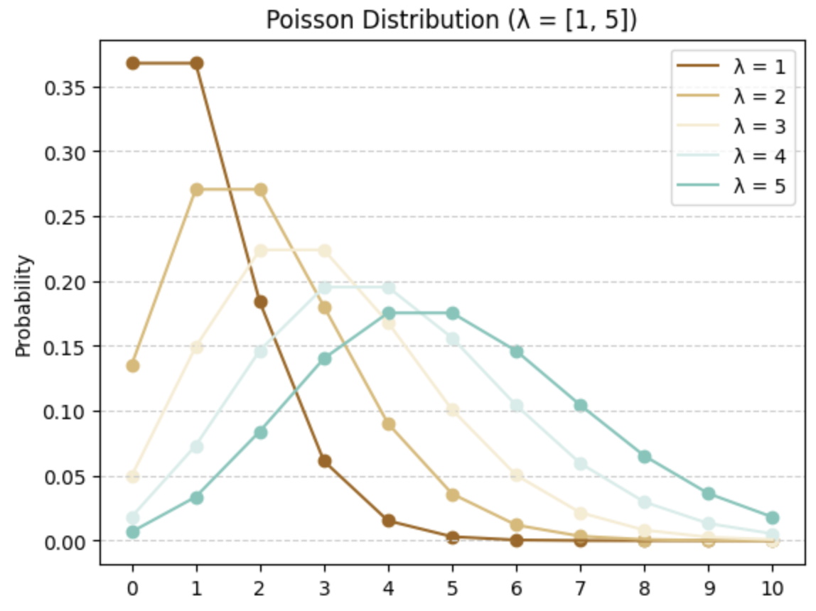
The Poisson distribution (단위 시간 안에 어떤 사건이 몇 번 발생할 것인지) provides the probability of the number of events occurring within a specific fixed interval, where the known constant rate of each event’s occurrence is represented by the symbol $\lambda$. The Poisson Distribution’s PMF is

$P(X=k) = \frac{e^{- \lambda}\lambda^{k}}{k!}$

mean: $\mu = \lambda$
variance: $\sigma^2 = \lambda$

The Poisson distribution is commonly used to analyze counts over a continuous interval, like the number of website visits in a specific time period or the number of defects in a square foot of fabric. In contrast to the binomial distribution which is used for scenarios like coin flips with a probability $p$ of getting a head, the Poisson distribution is utilized for processes $X$ occurring at a rate represented by $\lambda$.

Following is the example of Poisson distribution.

• The number of customers arriving within a given period of time
• The number of cracks on a one-kilometer stretch of road
• The number of defects occurring during a given production time
• The number of births occurring in one day
• The number of vehicles passing through a tollgate during a certain time period
• The error rate of typos occurring while completing a single page
• The number of mutations occurring when DNA is exposed to a specific amount of radiation
• The number of pine trees in a forest where various kinds of trees grow within a specific area
• The number of earthquakes occurring with a magnitude above a certain threshold

(https://ko.wikipedia.org/wiki/%ED%91%B8%EC%95%84%EC%86%A1_%EB%B6%84%ED%8F%AC)

(https://datadoctorblog.com/2023/08/23/Py-Stat-Distribution-Poisson/)