Day25 Statistics Review (4)

📚 The Start of Recording TIL Summer ‘24 : Why Did I Start This Project? 🚀

🔔 Don't Miss: Continous Records of TIL '25 (Still On-Going!) 🌟

✨ A New Chapter in TIL '25: Reflecting, Growing, and Moving Forward 📖

Population Proportions, p-values & Confidence Intervals, and Type I & II Errors

(Ace the Data Science Interview: 201 Real Interview Questions Asked By FAANG, Tech Startups, & Wall Street)

Hypothesis Testing for Population Proportions

The Central Limit Theorem (CLT) allows us to apply the Z-test to random variables of any distribution.

(For instance, when we want to estimate the sample proportion of a population with a specific characteristic, we can consider the population members as Bernoulli random variables, where those with the characteristic are represented by “1s” and those without it are represented by “0s”. We can then calculate the sample proportion by dividing the sum of these Bernoulli random variables by the total population size.)

From there, we can compute the sample mean and variance of the overall proportion and form the hypotheses accordingly.

$H_0: \hat{p}=p_0$
$H_1: \hat{p} \neq p_0$

and the corresponding test statistic to conduct a Z-test would be:

$z= \frac{\hat{p}-p_0}{\frac{p_0(1-p_0)}{n}}$

In practical terms, these test statistics are at the heart of A/B testing.

For example, let’s consider the previously discussed scenario where we want to measure conversion rates in groups A and B. Group A is the control group, and group B receives special treatment, such as a marketing campaign. Using the same null hypothesis as before, we can employ a Z-test to evaluate the difference in actual population means (in this case, conversion rates) and determine its statistical significance at a set level.

When discussing A/B testing or related topics, it’s important to always refer to the relevant test statistic and explain its validity (usually due to the Central Limit Theorem).

P-values and Confidence Intervals

P-values and confidence intervals are frequently discussed in various contexts. Put, a p-value represents the probability of observing the calculated test statistic value under the assumptions of the null hypothesis. Typically, the p-value is compared to a predetermined significance level ($\alpha$, often 0.05).

In a hypothesis test, we select a significance level, denoted as $\alpha$, as the acceptable probability of rejecting a true null hypothesis. We can calculate a confidence interval to evaluate the test statistic. This interval represents a range of values that, if a large sample were taken, would encompass the parameter value of interest 95% of the time (assuming a 95% confidence interval). If the confidence interval includes 0, we cannot reject the null hypothesis; if it doesn’t include 0, we can reject the null hypothesis.

The general form for a confidence interval around the population mean is as follows:

$\mu \pm z_{a/2} \frac{\sigma}{\sqrt{n}}$
where the term $z$ is the critical value
for the standard normal distribution.

With A/B testing on conversion rates, the confidence interval for a population proportion would be:

$\hat{p} \pm z_{a/2} \sqrt{\frac{\hat{p}(1-\hat{p})}{n}}$

since our estimate of the true proportion will have the following parameters when estimated as approximately Gaussian:

$\mu= \frac{np}{n}=p, \sigma^2 = \frac{np(1-p)}{n^2}=\frac{p(1-p)}{n}$

As long as the sampling distribution of a random variable is known, the appropriate p-values and confidence intervals can be assessed.

Type I and II Errors

Two common errors are often evaluated in statistical testing: type I error, also known as a “false positive,” and type II error, known as a “false negative.” Specifically, a type I error occurs when the null hypothesis is rejected incorrectly, and a type II error occurs when the null hypothesis is not rejected when it is actually incorrect.

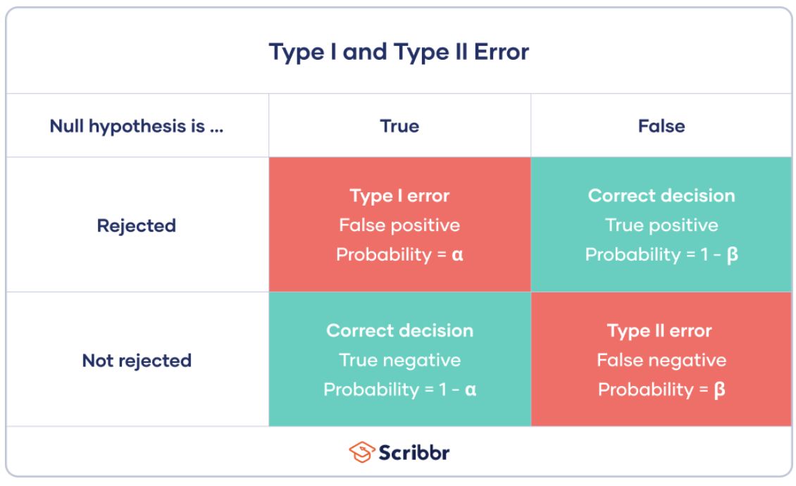
(https://www.scribbr.com/statistics/type-i-and-type-ii-errors/)

The confidence level is often represented as $1-\alpha$, while power is represented as $1 - β$. When plotting sample size against power, a general trend is that a larger sample size corresponds to higher power. Assessing power can be helpful in determining the necessary sample size to detect a significant effect. Generally, tests are designed to have both $1 - α$ and $1 - β$ relatively high, typically at 0.95 and 0.8, respectively.

When conducting multiple hypothesis tests, there is a risk that even if a particular outcome for one experiment seems unlikely, we might still observe a statistically significant outcome at least once. For example, if we set the significance level (α) at 0.05 and run 100 hypothesis tests, we would expect around 5 of the tests to be statistically significant simply due to chance. However, it’s best to maintain an overall α of 0.05 for all 100 tests. This can be achieved by adjusting the α level for each test to α/n, where n is the number of hypothesis tests (in this case, α/n = 0.05/100 = 0.0005). This adjustment is known as the Bonferroni correction, and it helps ensure that the overall rate of false positives is controlled within a multiple-testing framework.