Day30 ML Review - Logistic Regression (2)

📚 The Start of Recording TIL Summer ‘24 : Why Did I Start This Project? 🚀

🔔 Don't Miss: Continous Records of TIL '25 (Still On-Going!) 🌟

✨ A New Chapter in TIL '25: Reflecting, Growing, and Moving Forward 📖

Cost Function of Logistic Regression

Learning the Weights of the Logistic Cost Function

In logistic regression, the weights (or parameters) are crucial in determining the decision boundary that separates the classes. During training, the weights are optimized to minimize the logistic cost function, which evaluates how closely the model’s predictions align with the actual class labels.

The logistic cost function, also known as the log-loss or binary cross-entropy loss, is used to evaluate the performance of a logistic regression model. It is defined as follows:

For a single training example, the cost function $J(\theta)$ is given by: $ J(\theta) = - \left[ y \log(h_\theta(x)) + (1 - y) \log(1 - h_\theta(x)) \right] $

For a dataset with $m$ training examples, the overall cost function is the average of the individual costs: $ J(\theta) = \frac{1}{m} \sum_{i=1}^{m} \left[ - y^{(i)} \log(h_\theta(x^{(i)})) + (1 - y^{(i)}) \log(1 - h_\theta(x^{(i)})) \right] \ $

Here:

• $ \theta$ represents the vector of weights.
• $y^{(i)}$ is the true label for the $(i)^{th}$ training example.
• $x^{(i)}$is the feature vector for the $(i)^{th}$ training example.
• $h_\theta(x^{(i)}) = \sigma(\theta^T x^{(i)})$ is the predicted probability that the output is 1, given by the sigmoid function $\sigma(z) = \frac{1}{1 + e^{-z}}$.

Role of Weights

The weights $\theta = (\theta_0, \theta_1, \ldots, \theta_n)$ determine the influence of each feature $x_j$ on the predicted probability $ h_\theta(x) $. Specifically:

• $\theta_0$ is the intercept (bias term).
• $ \theta_1, \theta_2, \ldots, \theta_n $ are the coefficients for the respective features $ x_1, x_2, \ldots, x_n $.

The weights in logistic regression are important parameters that determine the classifier’s decision boundary. They are optimized by minimizing the logistic cost function using gradient descent or other optimization techniques, potentially with regularization to prevent overfitting.

(Python Machine Learning: Machine Learning and Deep Learning with Python, scikit-learn, and TensorFlow 2, 3rd Edition)

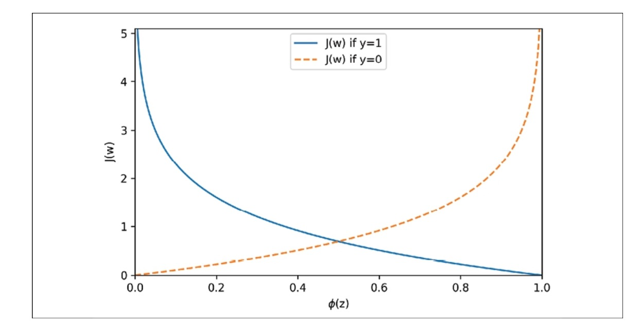
The cost approaches 0 on the y-axis if we correctly predict that an example belongs to class 1. Similarly, the cost also approaches 0 if we correctly predict y=0. However, if the prediction is wrong, the cost goes toward infinity. The main point is that we penalize wrong predictions with an increasingly higher cost.