Day34 ML Review - Support Vector Machine (3)

📚 The Start of Recording TIL Summer ‘24 : Why Did I Start This Project? 🚀

🔔 Don't Miss: Continous Records of TIL '25 (Still On-Going!) 🌟

✨ A New Chapter in TIL '25: Reflecting, Growing, and Moving Forward 📖

Solving Nonlinear Problems - Using a Kernal SVM

Another reason SVMs are highly popular among machine learning practitioners because they can be easily kernelized to solve nonlinear classification problems.

(Python Machine Learning: Machine Learning and Deep Learning with Python, scikit-learn, and TensorFlow 2, 3rd Edition)

Kernel Methods for Non-Linearly Data

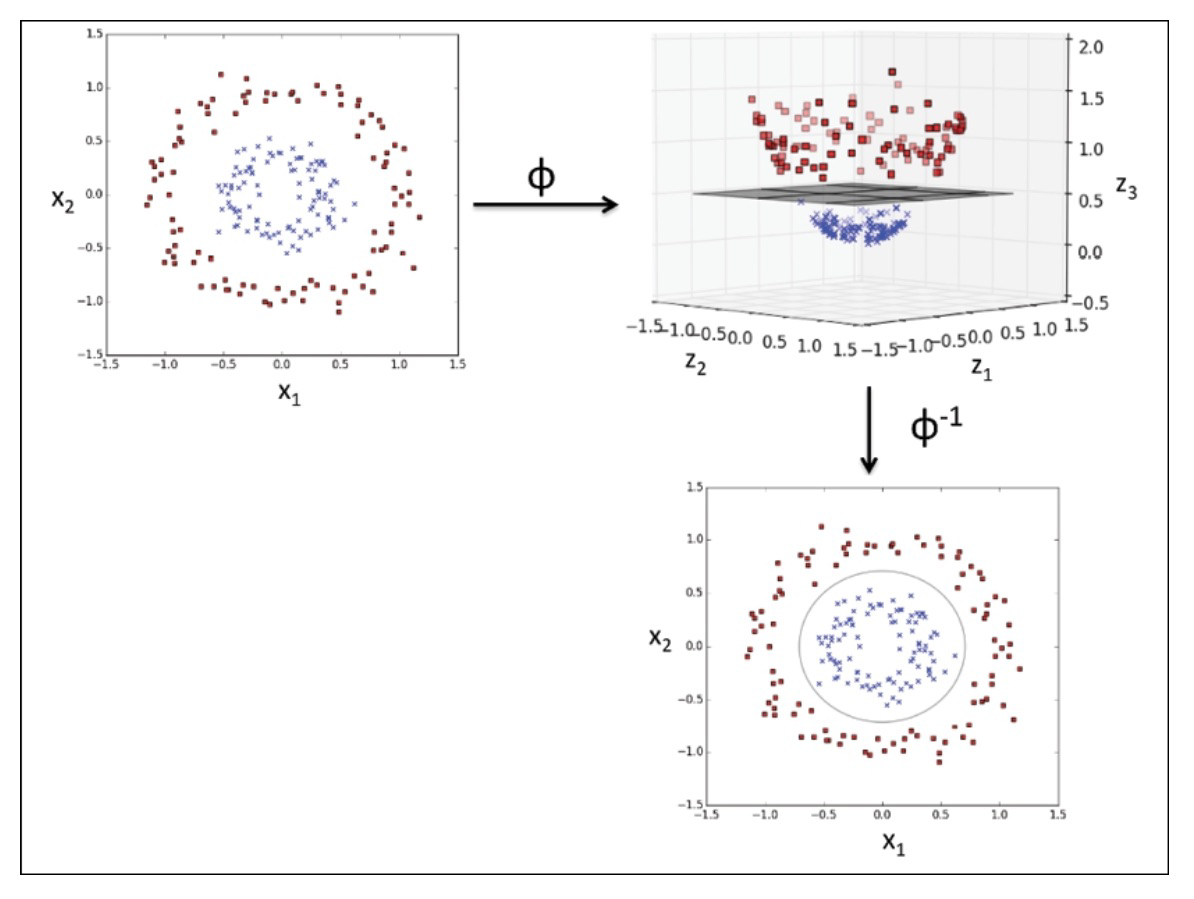
Kernel methods allow us to handle non-linearly separable data by creating nonlinear combinations of the original features. This is done by projecting the data onto a higher-dimensional space using a mapping function denoted as $\phi$, where the data becomes linearly separable. This process can transform a two-dimensional dataset into a new three-dimensional feature space, where the classes become separable via the following projection.

$\phi(x_1, x_2) = (z_1, z_2, z_3) = (x_1, x_2, x_1^2+x_2^2)$


(Python Machine Learning: Machine Learning and Deep Learning with Python, scikit-learn, and TensorFlow 2, 3rd Edition)

We can separate the two classes in the plot using a linear hyperplane, and this boundary becomes nonlinear when projected back onto the original feature space.

Using the Kernal Trick to Find Separating Hyperplanes in a High-Dimensional Space

We transform training data into a higher-dimensional feature space using a mapping function $\phi$ and train a linear SVM model. Using the linear SVM model, we then use the same mapping function to transform new, unseen data for classification. However, creating new features is computationally expensive, especially with high-dimensional data. This is where the so-called “kernel trick” becomes crucial.

Although we did not go into much detail about how to solve the quadratic programming task to train an SVM, in practice, we need to replace the dot product $x^{(i)T}x^{(j)}$ by $\Phi(x^{(i)})^T \Phi(x^{(j)})$. To save the expensive step of calculating this dot product between two points explicitly, we define a so-called Kernel Function:

$\kappa(x^{(i)}, x^{(j)}) = \Phi(x^{(i)})^T \Phi(x^{(j)})$

One of the most widely used kernels is the radial basis function (RBF) kernel, which can be called the Gaussian kernel:

$\kappa(x^{(i)}, x^{(j)}) = \exp\left(-\frac{\|x^{(i)} - x^{(j)}\|^2}{2\sigma^2}\right)$
$\rightarrow $ $\kappa(x^{(i)}, x^{(j)}) = \exp\left(-\gamma\|x^{(i)} - x^{(j)}\|^2\right)$

Here, $\gamma = \frac{1}{2\sigma^2}$ is a free parameter to be optimized.

The term “kernel” essentially represents a similarity function between two examples. The minus sign inverts the distance measure to produce a similarity score. As a result of the exponential term, the similarity score ranges between 1 (for exactly similar examples) and 0 (for dissimilar examples).

svm = SVD(kernel='rbf', random_state=1, gamma=0.10, C=10.0)
svm.fit(X_xor, y_xor)

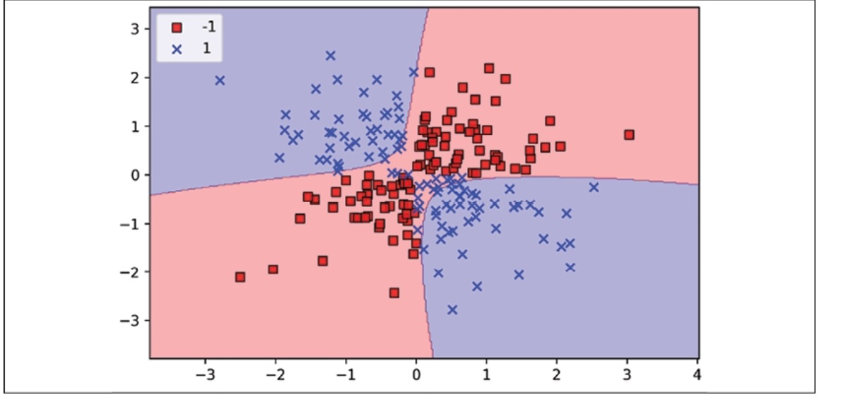
With gamma value 0.10

The $\gamma$ parameter, which we set to gamma=0.1, can be understood as a cutoff parameter for the Gaussian sphere. If we increase the value for gamma, we increase the influence or reach of the training examples, resulting in a tighter and more irregular decision boundary.

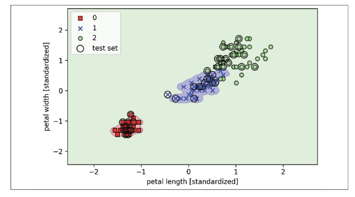
With gamma value 100

Although the model fits the training dataset very well, a classifier like this is likely to perform poorly on new, unseen data. This shows that the gamma parameter also plays a crucial role in controlling overfitting or variance when the algorithm is too sensitive to fluctuations in the training dataset.