
Day04 Basic Mathematics Review (4)
Bayesian Statistics, the Law of Total Probability, and Var-Cov Matrix

Bayesian Statistics
Bayesian Statistics is a subset of statistics in which probability expresses a degree of belief in an event. This belief may change as new evidence is presented. Bayesian statistics uses the Bayes theorem to update the probability of a hypothesis as more evidence or information becomes available.
In Bayesian statistics:
- Prior Probability represents what is initially believed before any evidence is introduced.
- Likelihood represents how probable new evidence is, given the prior.
- Posterior Probability is the updated belief after considering the new evidence.
The mathematical formula of Bayes theorem is: \(P(A \mid B) = \frac{P(B \mid A) \times P(A)}{P(B)}\)
- $P(A)$ is the prior probability of the hypothesis before seeing the evidence.
- $P(B \mid A)$ is the likelihood of observing the evidence $B$ given that $A$ is true.
- $P(A \mid B)$ is the posterior probability of the Hypothesis $A$ given the evidence $B$.
- $P(B)$ is the probability of the evidence under all possible hypotheses.
If this conditional probability is presented simply $P(A)$ - that is, if $P(A \mid B) = P(A)$, then $A$ and $B$ are independent.
The Bayesian rule is extremely important in real-life applications if other information is unavailable. For example, Bayes’ rule is especially important in medical testing for rare diseases since diagnosing someone with a disease may be misleading.
Bayes’ rule plays a crucial part in machine learning. Frequently, the goal is to identify the best conditional distribution for a variable given the available data.
Law of Total Probability
Assume we have several disjoint events within $B$ having occurred, we can then break down the probability of an event $A$ having also occurred thanks to the law of total probability, which is stated as follows:
This equation is so handy to use. If we want to model the probability of an event $A$ happening, it can be decomposed into the weighted sum of conditional probabilities based on each possible scenario having occurred. One common example is the probability that a customer makes a purchase, conditional on which customer segment that customer falls within.
Var-Cov Matrix
The variance-covariance matrix (often abbreviated as var-cov matrix is a key concept in statistics, particularly in the study of data distributions, linear regression, and multivariate analysis. This matrix provides a systematic way to capture the variances and covariances associated with multiple variables.
For a set of variables $X_n$ :
- The Variance of a variable measures the spread of its values from the mean, indicating how much the values differ from the mean.
- The Covariance measures how two variables change together, indicating the extent to which one variable increases as the other increases.
\(\begin{bmatrix}
\text{Var}(X_1) & \text{Cov}(X_1, X_2) & \dots & \text{Cov}(X_1, X_n) \\
\text{Cov}(X_2, X_1) & \text{Var}(X_2) & \dots & \text{Cov}(X_2, X_n) \\
\vdots & \vdots & \ddots & \vdots \\
\text{Cov}(X_n, X_1) & \text{Cov}(X_n, X_2) & \dots & \text{Var}(X_n)
\end{bmatrix}\)
The Var-Cov Matrix for $n$ variables is a $n \times n$ symmetric matrix where:
- The diagonal entries are the variances of each variable.
- The off-diagonal entries are the covariances between pairs of variables.
The covariance matrix of a random vector $X$ is defined as:
\(cov(X) = E[(X-E[X])(X-E[X])^T]\)
Where:
- $X$ is a matrix whose columns represent different variables (or random vectors).
- $E[X]$ is the expected value (mean) of $X$, usually calculated column-wise.
- $(X-E[X])$ represents the deviation of $X$ from its mean.
- $T$ denotes its transpose opration.
Calculation:
- Calculate $X-E[X]$: Each element of $X$ is subtracted by the mean of its respective column to get the deviation of each element from the mean.
- Transpose and Matrix Multiplication: $(X-E[X])$ is multiplied by its transpose $(X-E[X])^T$. This operation results in a square matrix where each element represents the covariance between different pairs of variables.
- Element-wise Computation in the Matrix: The matrix $E[(X-E[X])(X-E[X]^T)]$ is computed by taking the dot product of the rows of $X-E[X]$ with the columns of its transpose. This operation aggregates the product of deviations for each pair of variables across all observations.
- Taking Expectations (average): The expected value of the resulting matrix from step 3 is computed. Since expectation in the context of sample covariance is often approximated by the average, we divide the matrix element by the number of observations (or one less than the number of observations in some definitions, particularly for an unbiased estimate of sample covariance).
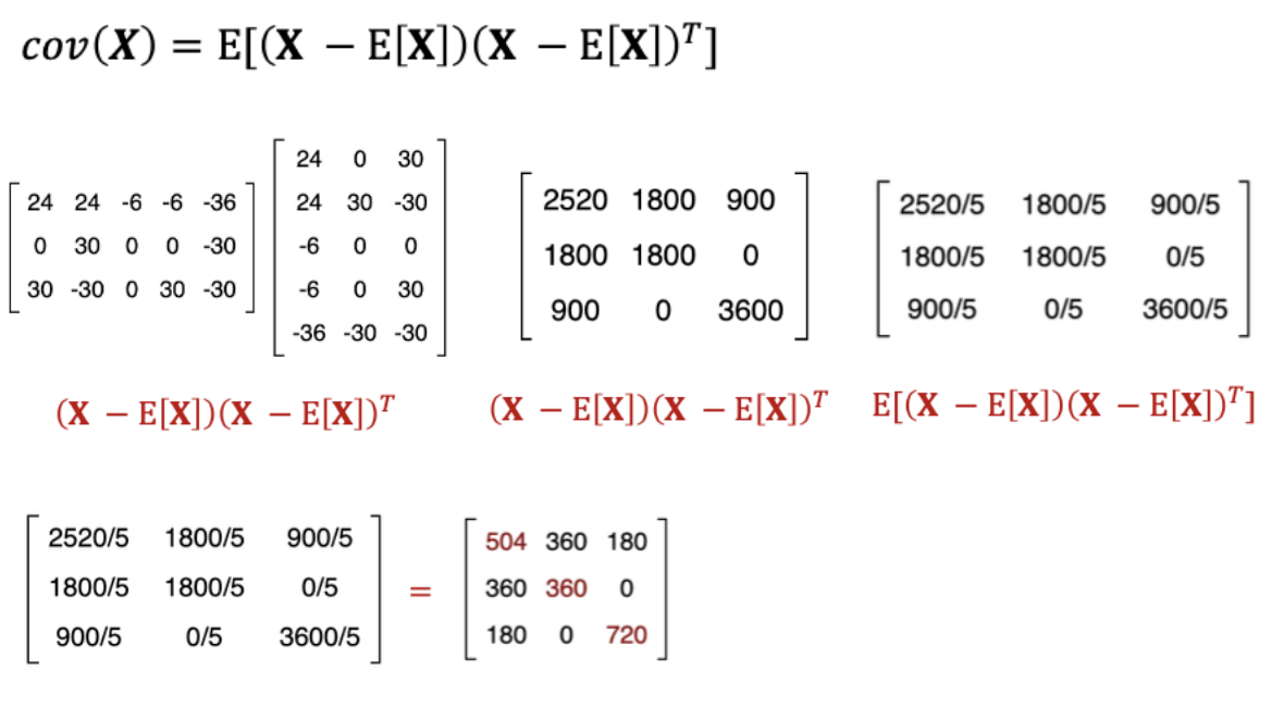
Therefore, for instance, the final matrix shown is:
- Diagonal entries (e.g., 504, 360, 720) represent the variance of each individual variables
- Off-diagonal entries (e.g., 360, 180, 0) represent the covariance between different pairs of variables, indicating how much two variables change together. A covariance of zero suggests no linear relationship.

Leave a comment