Day05 ML Review - Principle Component Analysis (1)

📚 The Start of Recording TIL Summer ‘24 : Why Did I Start This Project? 🚀

🔔 Don't Miss: Continous Records of TIL '25 (Still On-Going!) 🌟

✨ A New Chapter in TIL '25: Reflecting, Growing, and Moving Forward 📖

Mathematical Definition & Algorithms

PCA is a method for analyzing the main components of a distribution formed by multiple data sets rather than analyzing all of the components of each piece of data individually. It is widely used for dimensionality reduction in Machine Learning.

All explanation is mainly from The Dark Programer’s blog (https://darkpgmr.tistory.com/110)

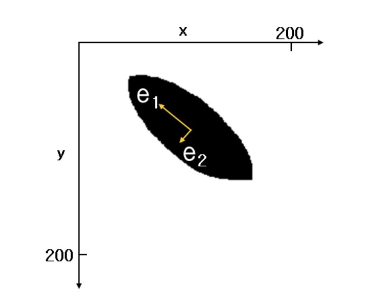
The best way to describe the distribution characteristics of these datasets is to explain them using two vectors, e1 and e2, as shown in the figure. Knowing the direction and size of e1 and e2 is the simplest and most effective way to understand this data distribution.

When we talk about ‘main components ‘, we’re referring to the directions in which the data’s variance is most significant. In other words, these are the paths along which the data spreads out the most. In Figure 1, you can see that the data’s dispersion, or degree of spread, is greatest along the e1 direction. The direction perpendicular to e1 and with the subsequent greatest dispersion of data is e2.

Straight-line approximation in 2-dimensional area

The PCA method for approximating a straight line involves deriving a line parallel to the first principal component vector from PCA while passing through the average position of the data.

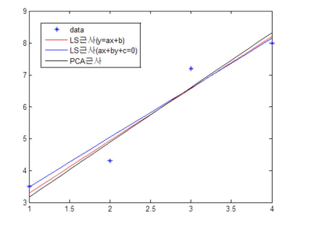
The straight line obtained from the PCA method differs from the one obtained from the Least Squares (LS) Method. The LS method minimizes the distance between a straight line and the data, while the PCA method identifies the direction in which the data has the greatest variance.

In the figure above, the LS approximation $y=ax+b$ minimizes the $y-axis$ distance from the straight line, and the other LS approximation $ax+by+c=0$ minimizes the $z-axis$ distance from plane $z=ax+by+c$. We need to select a straight line that maximizes the variance of the data among the lines that pass through the data’s average point when the data is projected.

PCA Mathematics

We need to determine the Covariance and Covariance Matrix before we can examine the detailed mathematics of the PCA.

• Covariance: Covariance measures the joint variability of two random variables. With the two variables, $x$ & $y$, $cov(X, Y)$​​ is as below.
  

  $$ \begin{align} cov(X,Y) = E[(X-E[X])(Y-E[Y])] \end{align} $$

  
  

  For two jointly distributed real-valued random variables $X$ and $Y$, the covariance is defined as the expected value (or mean) of the product of their derivations from their individual expected values. (https://en.wikipedia.org/wiki/Covariance)

• Covariance Matrix: A covariance matrix is a square matrix giving the covariance between each pair of elements of a given random vector. Any covariance matrix is symmetric and positive semi-definite, and its main diagonal contains variances.
  

  $$ C = \begin{pmatrix} \text{cov}(x,x) & \text{cov}(x,y) \\ \text{cov}(x,y) & \text{cov}(y,y) \end{pmatrix} $$

  
  

  $$ = \begin{pmatrix} \frac{1}{n} \sum (x_i - m_x)^2 & \frac{1}{n} \sum (x_i - m_x)(y_i - m_y) \\ \frac{1}{n} \sum (x_i - m_x)(y_i - m_y) & \frac{1}{n} \sum (y_i - m_y)^2 \end{pmatrix} $$

  
  PCA can be viewed as the process of eigendecomposition of the covariance matrix of input data into its eigenvectors and eigenvalues.

How the PCA works (e.g., in two dimensions)

1. Standardize the data:

   Subtract the mean of each feature in the dataset from all data points and then divide by the standard deviation. This ensures that each feature contributes equally to the analysis.
   

2. Compte the covariance matrix:

   For instance, for two dimensions, the covariance matrix $C$ is a $2 \times 2$ matrix where each element represents the covariance between two variables. The diagonal elements represent the variance of each variable, and the off-diagonal elements are the covariance as above.
   

3. Calculate Eigenvalue and Eigenvector:

   The covariance matrix is symmetric and real, so it can be diagonalized by finding its eigenvalues and eigenvectors. (The eigenvalues represent the variance explained by each principal component, and the eigenvectors represent the directions of these principal components.)
   

   $$ \text C \mathbf{v}_i = \lambda_i \mathbf{v}_i $$
   where $\mathbf{v_i} $ are the eigenvectors and $\lambda_i$ are the eigenvalues.
   

   
   

4. Choose Principal Components:

   In two dimensions, there are two principal components. The eigenvector associated with the larger eigenvalue is the first principal component (PC1). This represents the direction along which the data’s variance is maximized. The second principal component (PC2) is orthogonal to the first and represents the next highest variance direction.
   

5. Project the Data onto the Principal Components:

   Project the original data points onto the principal components to transform the data into the new subspace. This is done by multiplying the original data matrix (after standardization) by the matrix of eigenvectors.
   

\[Projected\ Data = Data\ Matrix\ \times \ Eigenvector\ Matrix\]

Example of calculation

Let’s assume that after calculating the covariance, we got the result below.

$$ C = \begin{bmatrix} 1 & 0.8 \\ 0.8 & 1 \end{bmatrix} $$

To find the eigenvalues $\lambda$ and eigenvectors $\mathbf{v}$ of $C$, we solve the characteristic equation.

$$ det(\text C - \lambda \text I) \\ $$
where $I$ is the identity matrix.

Substituting $\text C$ and $\text I$, the equation becomes:

$$ det \left(\begin{bmatrix} 1 - \lambda & 0.8 \\ 0.8 & 1 - \lambda \end{bmatrix}\right) = 0 $$

The determinant of this matrix is calculated as:

$$ (1 - \lambda)(1 - \lambda) - (0.8)(0.8) = \lambda^2 - 2\lambda + 1 - 0.64 = \lambda^2 - 2\lambda + 0.36 $$

Setting this equal to zero and solving for $\lambda$​ :

$$ \lambda^2 - 2\lambda + 0.36 = 0 $$

$$ \lambda = \frac{2 \pm \sqrt{4 - 1.44}}{2} = \frac{2 \pm \sqrt{2.56}}{2} = \frac{2 \pm 1.6}{2} $$

$$ \lambda_1 = 1.8, \quad \lambda_2 = 0.2 $$

Find the Eigenvectors:

For $\lambda_1 = 1.8$:

$$ (\text C - 1.8 \text I)\mathbf{v} = 0 \\ $$
$$ \begin{bmatrix} -0.8 & 0.8 \\ 0.8 & -0.8 \end{bmatrix} \begin{bmatrix} x \\ y \end{bmatrix} = \begin{bmatrix} 0 \\ 0 \end{bmatrix} $$

$$ x = y $$

Choose $x=1$, then $y=1$, leading to the eigenvector:

$$ \mathbf{v}_1 = \frac{1}{\sqrt{2}}\begin{bmatrix} 1 \\ 1 \end{bmatrix} $$

For $\lambda_2 = 0.2$:

$$ (\text C - 0.2 \text I)\mathbf{v} = 0 $$

$$ \begin{bmatrix} 0.8 & 0.8 \\ 0.8 & 0.8 \end{bmatrix} \begin{bmatrix} x \\ y \end{bmatrix} = \begin{bmatrix} 0 \\ 0 \end{bmatrix} $$

$$ x = -y $$

Choose $x=1$, then $y=-1$, leading to the eigenvector:

$$ \mathbf{v}_2 = \frac{1}{\sqrt{2}}\begin{bmatrix} 1 \\ -1 \end{bmatrix} $$

The principal components are:

• $\mathbf{v_1}$ associated with $\lambda_1=1.8$, which indicates the direction of maximum variance.
• $\mathbf{v_2}$ associated with $\lambda_2=0.2$, which is orthogonal to $\mathbf{v_1}$, and indicates the direction of the least variance.

Then, we multiply this Eigenvector Matrix with the Data matrix.