
Day50 ML Review - Dimensionality Reduction (1)
Compressing Data via Dimensionality Reduction and Summary of PCA

In my earlier articles, I talked about different methods for decreasing the dimensionality of a dataset through various feature selection techniques. Another way to achieve dimensionality reduction is through feature extraction.
To conduct feature extraction, it’s crucial to convert the data in a dataset into a new feature subspace with lower dimensionality than the original. Data compression is vital, enabling us to store and analyze the growing volume of generated and gathered data.
In summary, there are three principal methodologies for data compression:
- Principal Component Analysis (PCA): for unsupervised data compression. We discussed it before.
- Linear Discriminant Analysis(LDA): as a supervised dimensionality reduction technique for maximizing class separability.
- Nonlinear dimensionality reduction via Kernel Principal Component Analysis (KPCA).
Principal Component Analysis (PCA)
We have discussed this subject frequently in my previous posts here:
- Day05 ML Review - Principle Component Analysis (1)
- Day06 ML Review - Principle Component Analysis (2)
- Day18 ML Review - Principle Component Analysis (3)
To recap those ideas, just like feature selection, we have various feature extraction methods at our disposal to decrease the number of features in a dataset. Feature selection involves retaining the original features, as seen in algorithms like Sequential Backward Selection, while feature extraction entails transforming or projecting the data onto a new feature space. The feature extraction process enhances data storage capacity and predictive accuracy by addressing the curse of dimensionality, particularly in the case of non-regularized models.
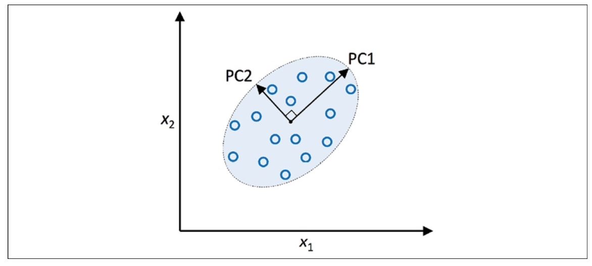
PCA enables us to recognize data patterns by examining the relationships between features. Simply put, PCA is designed to discover the most variable directions in data with many dimensions and then map the data onto a new space with the same number or fewer dimensions. The perpendicular axes (principal components) in the new space represent the most variable directions, considering that the new feature axes are perpendicular to each other, as shown in the illustration below:
When PCA is employed for reducing dimensionality, we create a transformation matrix, $W$, with dimensions $d \times k$. This matrix enables us to transform a vector, $x$, representing the features of a training example in a new $k$-dimensional feature subspace with fewer dimensions than the original d-dimensional feature space.
After transforming the original $d$-dimensional data to a new $k$-dimensional subspace, PC1 will have the highest variance possible. All subsequent principal components will have the greatest variability while being uncorrelated (orthogonal) to the other principal components. The resulting principal components will be mutually orthogonal (uncorrelated) even if the input features are correlated. PCA directions are greatly influenced by data scaling, and it’s necessary to standardize the features before PCA if the features were measured on different scales and equal importance needs to be assigned to all features.
PCA follows the steps below.
- Make the dataset with $d$ dimensions standardized.
- Create the matrix for covariance.
- Break down the covariance matrix into its eigenvectors and eigenvalues.
- Arrange the eigenvalues in descending order to prioritize the corresponding eigenvectors.
- Choose $k$ eigenvectors, which correspond to the $k$ largest eigenvalues, where $k$ $\leq$ $d$.
- Build a projection matrix, $W$, from the “top” $k$ eigenvectors.
- Use the projection matrix, $W$, to transform the $d$-dimensional input dataset $X$ and obtain the new $k$-dimensional feature subspace.
Let’s perform the PCA algorithm step by step using scikit-learn with the wine dataset.
1. Standardize the dataset
import pandas as pd
from sklearn.model_selection import train_test_split

# Split the dataset
X_train, X_test, y_train, y_test = train_test_split(X, y, test_size=0.3,
                                                   stratify=y,
                                                   random_state=0)

# Standardize the features
from sklearn.preprocessing import StandardScaler
sc = StandardScaler()
X_train_std = sc.fit_transform(X_train)
X_test_std = sc.transform(X_test)
2. Create the covariance matrix
The covariance matrix is symmetrical and has $d \times d$ dimensional dimensions, where $d$ represents the number of dimensions in the dataset. It contains the pairwise covariances between the various features. (note that if the dataset is standardized, the sample means are zero). A positive covariance means features increase or decrease together, while a negative covariance means features vary in opposite directions.
The eigenvectors of the covariance matrix represent the principal components (the directions of maximum variance), whereas the corresponding eigenvalues will define their magnitude.
3. Find eigenpairs of the covariance matrix
An eigenvector, $v$, satisfies the following condition:
where $\lambda$ is a scalar (the eigenvalue)
We can use linalg.eig function from NumPy to obtain the eigenpairs of the Wine covariance matrix.
import numpy as np
cov_mat = np.cov(X_train_std.T)
eigen_vals, eigen_vecs = np.linalg.eig(cov_mat)
We used numpy.cov to compute the covariance matrix of the standardized training dataset. Then, we used linalg.eig to perform eigendecomposition, which resulted in a vector (eigen_vals) with 13 eigenvalues and the corresponding eigenvectors stored as columns in a $13 \times 13$ dimensional matrix (eigen_vecs).
4. Arrange the eigenvalues in descending order
The key to reducing its dimensionality by projecting it onto a new feature space is selecting a subset of the eigenvectors, also known as principal components, that contains the most valuable information regarding the dataset’s variance. The eigenvalues provide us with the magnitude of the eigenvectors and must be sorted in decreasing order to identify the top $k$ eigenvectors that are most important based on their corresponding eigenvalues.
# Make a list of (eigenvalue, eigenvector) tuples
eigen_pairs = [(np.abs(eigen_vals[i]), eigen_vals[:, i]) for i in range(len(eigen_vals))]

# Sort the (eigenvalue, eigenvector) tuples from high to low
eigen_pairs.sort(key=lambda k: k[0], reverse = True)
5. Choose $k$ eigenvectors, which correspond to the $k$ largest eigenvalues,
We will select the two eigenvectors corresponding to the two largest eigenvalues to capture approximately 60 percent of the variance in this dataset. It’s important to note that we have chosen two eigenvectors for illustrative purposes, as we will later plot the data using a two-dimensional scatter plot in this subsection. In real-world applications, the number of principal components must be determined by balancing computational efficiency with the classifier’s performance.
w = np.hstack((eigen_pairs[0][1][:, np.newaxis], eigen_pairs[1][1][:, np.newaxis]))
By executing the preceding code, we have created a $13 \times 2$ - dimensional projection matrix, $W$, from the top two eigenvectors.
6. Build a projection matrix, $W$, from the “top” $k$ eigenvectors.
Using the projection matrix, we can now transform an example, $x$ (represented as a 13-dimensional row vector), onto the PCA subspace (the principal components one and two), obtaining $x’$, now a two-dimensional example vector consisting of two new features: $x’ = xW$
X_train_std[0].dot(w)
7. Use the projection matrix, $W$, to transform the $d$-dimensional input dataset $X$
Similarly, we can transform the entire $124 \times 13$ - dimensional training dataset onto the two principal components by calculating the matrix dot product: $X’ = XW$
X_train_pca = X_train_std.dot(w)
Upon implementing the code above, it becomes evident that the data is more dispersed along the $x$-axis, representing the first principal component, than along the $y$-axis, thus aligning with the findings of the explained variance ratio plot.
Leave a comment