
Day51 ML Review - Dimensionality Reduction (2)
Compressing Data via Linear Discriminant Analysis

Linear Discriminant Analysis (LDA) is a powerful technique for extracting essential features from data. LDA aims to identify the feature subspace that maximizes the separation between classes.
This significantly improves computational efficiency and mitigates the overfitting issue that arises from the curse of dimensionality in non-regularized models.
Principle Component Analysis vs. Linear Discriminant Analysis
PCA and LDA are linear transformation techniques that can reduce the number of dimensions in a dataset. PCA is an unsupervised algorithm, whereas LDA is supervised. However, there are cases where PCA works well, such as in image classifiers.
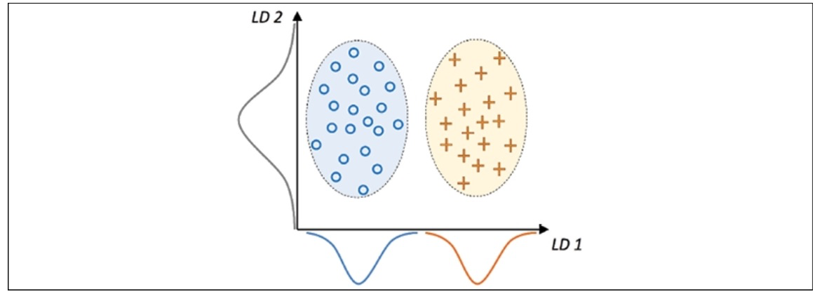
A linear discriminant, visually illustrated on the x-axis as LD 1, can effectively separate the two normally distributed classes. In contrast, the illustrated linear discriminant on the y-axis, known as LD 2, captures a substantial amount of the variance present in the dataset. However, it is not considered an effective linear discriminant since it does not encapsulate class-discriminatory information.
The LDA follows the steps below.
- Standardize the dataset with $d$ dimensions, where $d$ is the number of features.
- Calculate the mean vector with $d$ dimensions for each category.
- Create the between-class scatter matrix, $S_B$, and the within-class scatter matrix, $S_W$.
- Find the eigenvectors and their corresponding eigenvalues of the matrix $S^{-1}_{W}S_B$.
- Arrange the eigenvalues in descending order to determine the ranking of the corresponding eigenvectors.
- Select the $k$ eigenvectors that align with the $k$ largest eigenvalues to form a $d \times k$ -dimensional transformation matrix, $W$; these eigenvectors represent the columns of this matrix.
- Project the examples onto the new feature subspace using the transformation matrix, $W$.
The primary idea behind LDA closely resembles PCA because it involves decomposing matrices into eigenvalues and eigenvectors to create a new lower-dimensional feature space. However, LDA incorporates class label information through mean vectors computed in step 2.
1. Standardize the dataset
This step works in the same way as PCA.
import pandas as pd
from sklearn.model_selection import train_test_split

# Split the dataset
X_train, X_test, y_train, y_test = train_test_split(X, y, test_size=0.3,
                                                   stratify=y,
                                                   random_state=0)

# Standardize the features
from sklearn.preprocessing import StandardScaler
sc = StandardScaler()
X_train_std = sc.fit_transform(X_train)
X_test_std = sc.transform(X_test)
2. Calculate the mean vector
We will proceed by computing the average vectors, which we will utilize to form the within-class scatter matrix and between-class scatter matrix accordingly. Each average vector is denoted as $\mathbf m_i$, holds the mean feature value $\mu_m$ in relation to the examples of class $i$:
This results in three mean vectors:
np.set_printoptions(precision=4)
mean_vecs = []
for label in range(1,4):
  mean_vencs.append(np.mean(X_train_std[y_train==label], axis=0))
  print('MV %s: %s\n' %(label, mean_vecs[label-1]))
3. Create the between-class $S_B$, and the within-class scatter matrix, $S_W$
Using the mean vectors, we can now compute the within-class scatter matrix, $S_W$.
This is calculated by summing up the individual scatter matrices, $S_i$, of individual class $i$:
d = 13 # number of features
S_W = np.zeros((d, d))
for label, mv in zip(range(1,4), mean_vecs):
  class_scatter = np.zeros((d, d))
for row in X_train_std[y_train == label]:
  row, mv = row.reshaped(d, 1), mv.reshaped(d, 1)
  class_scatter += (row - mv).dot((row - mv).T)
  S_W += class_scatter
print('Within-class scatter matrix: %sx%s' %(S_W.shape[0], S_W.shape[1]))
The computation of scatter matrices assumes that the class labels in the training dataset are uniformly distributed. However, upon inspecting the number of class labels, it becomes evident that this assumption is not met.
As a result, it is necessary to scale the individual scatter matrices, $S_i$, before aggregating them into the scatter matrix $S_W$. Dividing the scatter matrices by the number of class examples, $n_i$ reveals that computing the scatter matrix is essentially equivalent to computing the covariance matrix, $\sum_i$. The covariance matrix can be viewed as a normalized version of the scatter matrix.
d = 13 # number of features
S_W = np.zeros((d, d))
for label,mv in zip(range(1, 4), mean_vecs):
  class_scatter = np.cov(X_train_std[y_train==label].T)
  S_W += class_scatter
print('Scaled within-class scatter matrix: %sx%s' % (S_W.shape[0], S_W.shape[1]))
After we compute the scaled within-class scatter matrix (or covariance matrix), we can move on to the next step and compute the between-class scatter matrix $\mathbf S_B$ :
Here, $m$ is the overall mean that is computed, including examples from all $c$ classes.
mean_overall = np.mean(X_train_std, axis=0)
d = 13 # number of features
S_B = np.zeros((d,d))
for i, mean_vec in enumerate(mean_vecs):
  n = X_train_std[y_train == i+1, :].shape[0]
  mean_vec = mean_vec.reshape(d, 1) #make column vector
  mean_overall = mean_overall.reshape(d, 1)
  S_B += n* (mean_vec - mean_overall).dot(
  (mean_vec - mean_overall).T)
print('Between-class scatter matrix: %sx%s' % (S_B.shape[0], S_B.shpae[1]))
4. Find the eigenvectors and their corresponding eigenvalues of the matrix $S^{-1}_{W}S_B$
The LDA’s remaining steps are similar to the PCA’s steps. Instead of conducting eigendecomposition on the covariance matrix, we use the generalized eigenvalue problem of the matrix, $S^{-1}_{W}S_B$.
eigen_vals, eigen_vec = np.linalg.eig(np.linalg.inv(S_W).dot(S_B))
5. Arrange the eigenvalues in descending order.
After we compute the eigenpairs, we can sort the eigenvalues in descending order.
eigen_pairs = [(np.abs(eigen_vals[i]), eigen_vecs[:,i]) for i in range(len(eigen_vals))]
eigen_pairs = sorted(eigen_pairs, key=lambda k: k[0], reverse=True)
print('Eigenvalues in descending order:\n') for eigen_val in eigen_pairs: print(eigen_val[0])
6. Select the $k$ eigenvectors with the $k$ largest eigenvalues to form a $d \times k$ -dimensional transformation matrix, $W$.
In Linear Discriminant Analysis (LDA), the maximum number of linear discriminants is limited to the number of class labels minus one. This limitation arises from the formation of the in-between scatter matrix, $\mathbf{S_B}$, which involves adding $c$ matrices, each of which has a rank of one or less. There are only two nonzero eigenvalues (note that the eigenvalues 3-13 are not precisely zero, but this results from floating-point arithmetic in NumPy).
w = np.hstack((eigen_pairs[0][1][:, np.newaxis].real, eigen_pairs[1][1][:, np.newaxis].isreal))
print("Matrix W: \n", w)
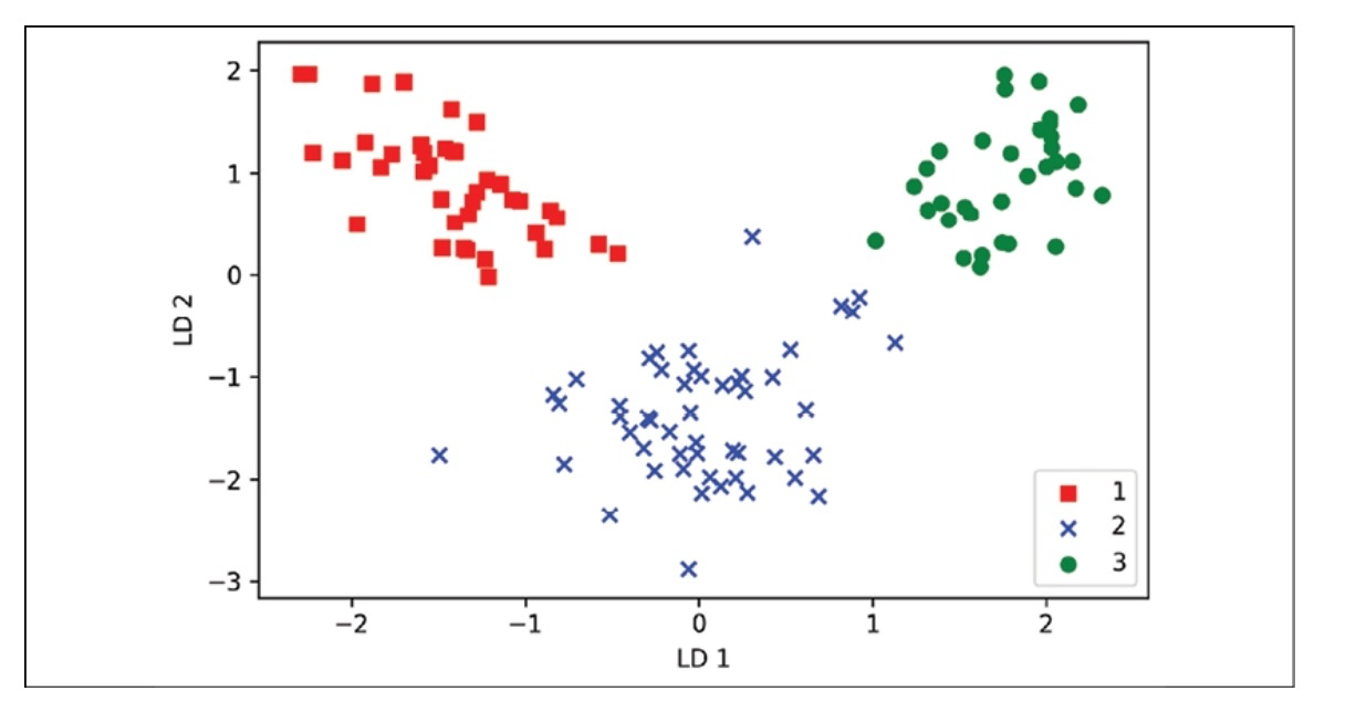
7. Project examples onto the new feature space
We will transform the training dataset by multiplying the following matrices using the transformation matrix, W.
X_train_lda = X_train_std.dot(w)

# to visualize this with a scatter plot
colors = ['r', 'b', 'g']
markers = ['s', 'x', 'o']
for l, c, m in zip(np.unique(y_train), colors, markers): plt.scatter(X_train_lda[y_train==1, 0], X_train_lda[y_train==1, 1]*(-1), c=c, label=1, marker=m)
plt.xlabel('LD 1')
plt.ylabel('LD 2')
plt.legend(loc='lower right')
plt.tight_layout()
plt.show()
Leave a comment