
Day53 ML Review - Dimensionality Reduction (4)
Implementing a Kernal Principal Component Analysis(KPCA) in Python

We are going to implement an RBF KPCA in Python for example.
from scipy.spatial.distance import pdist, squareform
from scipy import exp
from scipy.linalg import eigh
import numpy as np
def rbf_kernel_pca(X, gamma, n_components):
  """
  RBF kernel PCA implementation:
  X: {NumPy ndarray}, shape = [n_examples, n_features]
  gamma (float): Tuning parameter of the RBF kernel
  n_components (int): Number of principal components to return

  returns projected  dataset
  X_pc: {NumPy ndarray}, shape = [n_examples, k_features]
  """

  # Calculate pairwise squared Euclidean distances
  # in the MxN dimensional dataset.
  sq_dists = pdist(X. 'sqeuclidean')

  # Convert pairwise distances into a square matrix
  mat_sq_dists = squareform(sq_dists)

  # Compute the symmetric kernel matrix.
  K = exp(-gamma * mat_sq_dists)

  # Center the kernel matrix.
  N = K.shape[0]
  one_n = np.ones((N,N)) / N
  K = K - one_n.dot(K) - K.dot(one_n) + one_n.dot(K).dot(one_n)

  # Obtaining eigenpairs from the centered kernel matrix
  # scipy.linalg.eigh returns them in ascending order
  eigvals, eigvecs = eigh(K)
  eigvals, eigvecs = eigenvals[::-1], eigvecs[:, ::-1]

  # Collect the top k eigenvectors (projected examples)
  X_pc = np.column_stack([eigvecs[:, i] for i in range(n_components)

  return X_pc
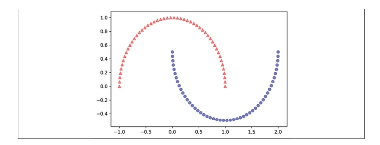
Example 1 - separating half-moon shapes
Let’s use our rbf_kernel_pca on various nonlinear example datasets. First, we’ll generate a 2D dataset with 100 sample points that depict two half-moon shapes.
from sklearn.datasets import make_moons
X, y = make_moons(n_samples = 100, random_state=123)
In the following diagram, you can see how the dataset transforms when using Standard PCA.
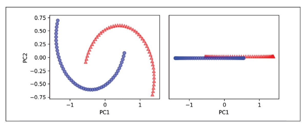
The original half-moon shapes appear slightly sheared and flipped across the vertical center. This transformation would not assist a linear classifier in distinguishing between circles and triangles. Similarly, if we project the dataset onto a one-dimensional feature axis, the circles and triangles corresponding to the two half-moon shapes are not linearly separable, as shown in the right subplot.
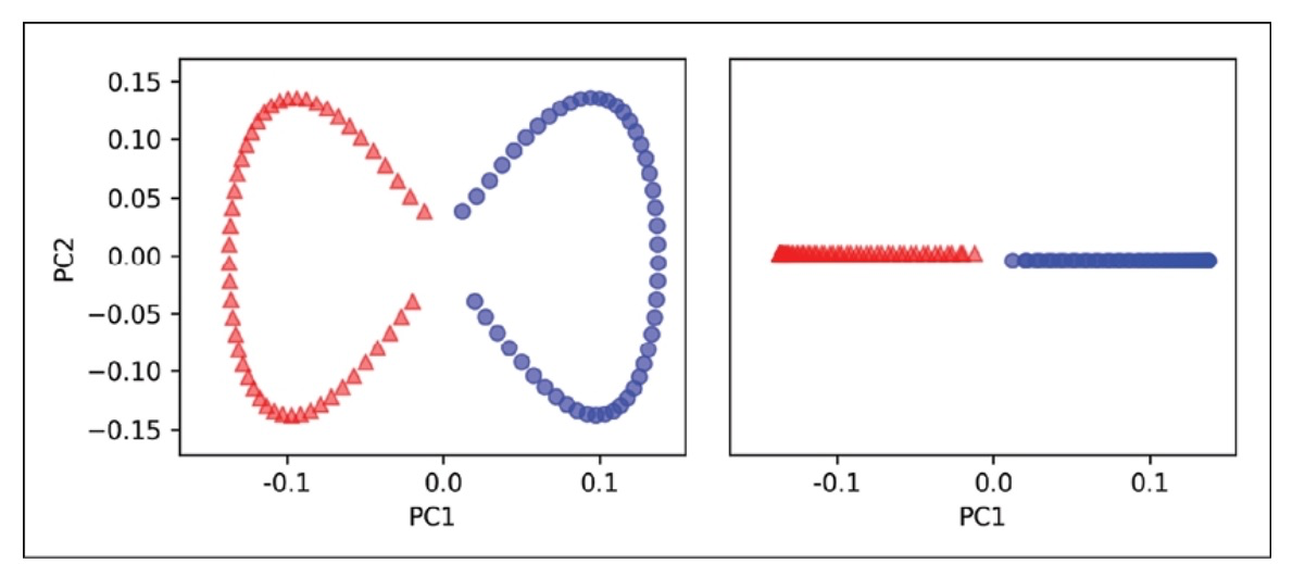
Let’s evaluate the performance of the rbf_kernel_pca method we implemented by following the steps below.
X_kcpa = rbf_kernel_pca(X, gamma=15, n_components=2)
The two categories (circles and triangles) are distinctly separated linearly, so we have an appropriate training dataset for linear classification.
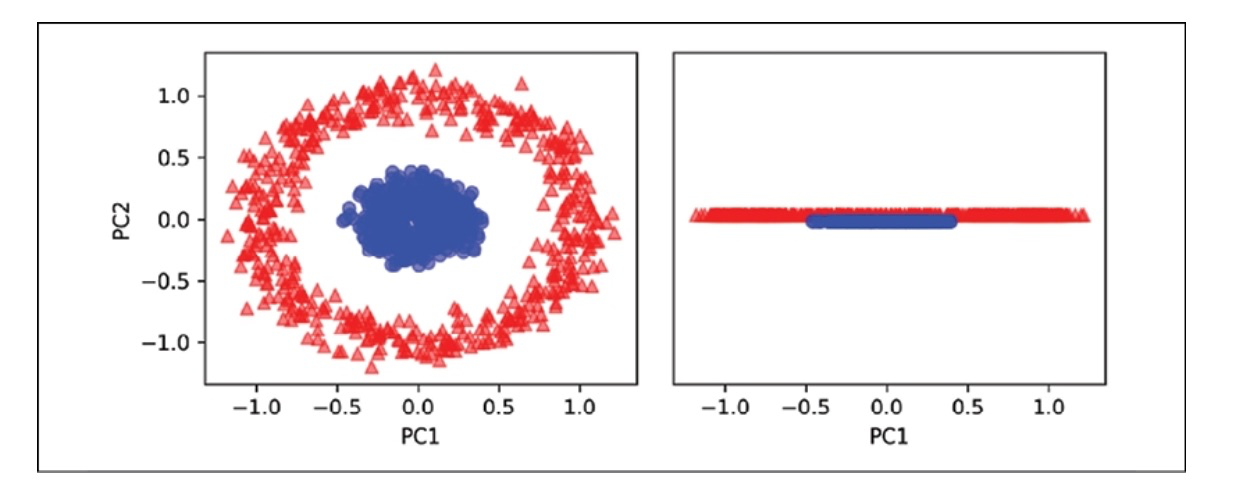
Example 2 - separating concentric circles
We will examine another instance of concentric circles using the following code.
from sklearn.datasets import make_circles
X, y = make_circles(n_samples = 1000, random_state=123, noise=0.1, factor = 0.2)
plt.scatter(X[y == 0, 0], X[y == 0, 1], color = 'red', marker='^', alpha = 0.5)
plt.scatter(X[y == 1, 0], X[y == 1, 1], color = 'blue', marker='o', alpha = 0.5)
plt.tight_layout()
plt.show()
The data will be represented below.

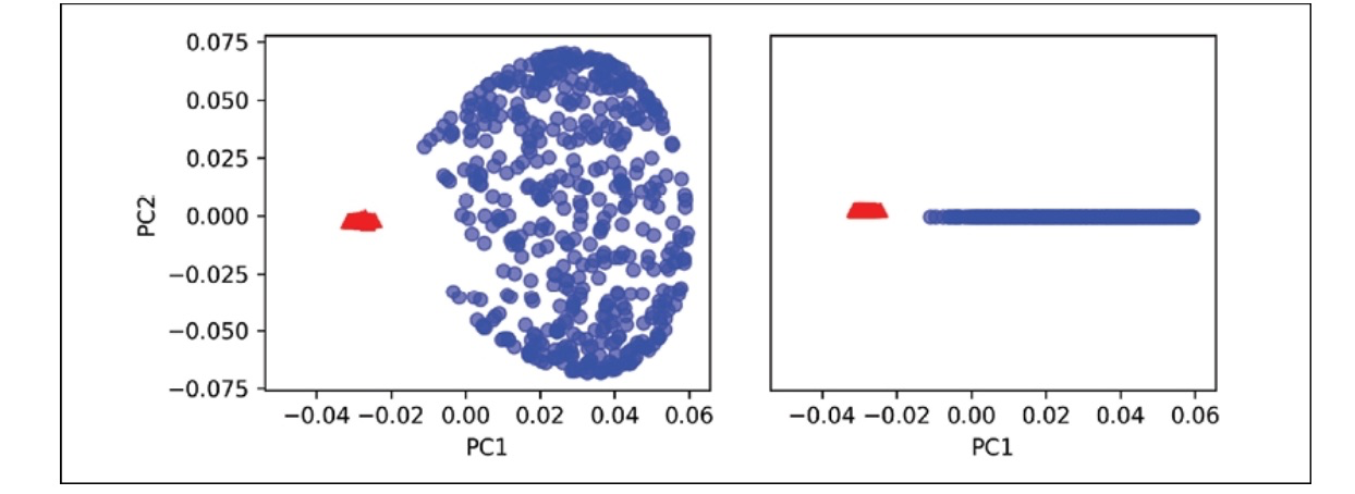
Begin by using the regular PCA method to contrast it with the outcome of the RBF kernel PCA.
scikit_pca = PCA(n_components = 2)
X_spca = scikit_pca.fit_transform(X)
We can see that standard PCA cannot produce results for training a linear classifier.
When we employ the rbf_kcpa technique, we notice that the data has been transformed into a new subspace where the two classes are now linearly separable.
X_kcpa = rbf_kernel_pca(X, gamma=15, n_components=2)
fig, ax = plt.subplots(nrows=1, ncols=2, gif-size=(7,3))
ax[0].scatter(X_kpca[y==0, 0], X_kpca[y==0, 1], color='red', marker='^', alpha=0.5)
ax[0].scatter(X_kpca[y==1, 0], X_kpca[y==1, 1], color='blue', marker='o', alpha=0.5)
ax[1].scatter(X_kpca[y==0, 0], np.zeros(500,1))+0.02, color='red', marker='^', alpha=0.5)
ax[1].scatter(X_kpca[y==1, 0], np.zeros(500,1))-0.02, color='blue', marker='o', alpha=0.5)
Leave a comment