Day54 ML Review - Dimensionality Reduction (5)

📚 The Start of Recording TIL Summer ‘24 : Why Did I Start This Project? 🚀

🔔 Don't Miss: Continous Records of TIL '25 (Still On-Going!) 🌟

✨ A New Chapter in TIL '25: Reflecting, Growing, and Moving Forward 📖

Applying Kernal Principal Component Analysis(KPCA) to New Data Points

In the previous post, we considered applying KPCA to two datasets: one with half-moon shapes and the other with concentric circles. In practical scenarios, we often need to transform multiple datasets, such as training and test data, and even new examples we gather after building and evaluating the model.

Remember that we can compute the following equation. An eigenvector($\alpha$) of the centered kernel matrix (not the covariance matrix), which means that those are the examples that are already projected onto the principal component axis, $v$. Thus, if we want to project a new example, $x’$, onto this principal component axis.

$\phi(x')^Tv$

KPCA (Kernel Principal Component Analysis) differs from standard PCA because it is a memory-based method. This means we need to use the original training dataset whenever we want to project new examples again. We have to calculate the pairwise RBF kernel (similarity) between each $i$th example in the training dataset and the new example, $x’$:

$\phi(x')^Tv = \sum_i a^{(i)} \phi (x')^T \phi (x^{(i)})$

$= \sum_i a^{(i)} \kappa (x', x^{(i)})$

In this context, the eigenvalues (represented by $\lambda$) and the corresponding eigenvectors (denoted as $\alpha $) of the kernel matrix $\mathbf K$ satisfy the following conditions within the given equation.

$\mathbf{K}a= \lambda a $

Following the process of measuring the similarity between the new examples and the examples in the training dataset, it is necessary to adjust the eigenvector, denoted as “$\alpha$” based on its corresponding eigenvalue. Hence, we should enhance the rbf_kernel_pca function that we previously developed to include the eigenvalues of the kernel matrix as part of its output.

Implementation in Python Step-by-Step

from scipy.spatial.distance import pdist, squareform
from scipi import exp
from scipy.linalg import eigh
import numpy as np
def rbf_kernel_pca(X, gamma, n_components):
  """
  RBF kernel PCA implementation.
  
  Parameters
  ------------
  X: {NumPy ndarray}, shape = [n_examples, n_features]
  
  gamma: float
  		Tuning parameter of the RBF kerneal
  		
  n_components: int
  		Number of principal components to return
  
  Returns
  -----------
  alphas {NumPy ndarray}, shape = [n_examples, k_features]
  		Projected dataset
  
  lambdas: list
  		Eigenvalues
 
  """
  # Calculate pairwise squared Euclidean dsitances
  # in the MxN dimensional dataset.
  sq_dists = pdist(X, 'sqeuclidean')
  
  # Convert pairwise distances into a square matrix
  mat_sq_dists = squareform(sq_dists)
  
  # Compute the symmetric kernel matrix.
  K = exp(-gamma * mat_sq_dists)
  
  # Center the kernal matrix.
  N = K.shape[0]
  one_n = np.ones((N,N)) / N
  K = K - one_n.dot(K) - K.dot(one_n) + one_n.dot(K).dot(one_n)
  
  # Obtaining eigenpairs from the centered kernel matrix
  # scipy.linalg.eigh returns them in ascending order
  eigvals, eigvecs = eigh(K)
  eigvals, eigvecs = eigvals[::-1], eigvecs[:, ::-1]
  
  # Collect the top k eigenvectors (projected examples)
  alphas = np.column_stack([eigvecs[:, i] for i in range(n_components)])
  
  # Collect the corresponding eigenvalues
  lambdas = [eigenvals[i] for i in range(n_components)]
  return alphas, lambdas

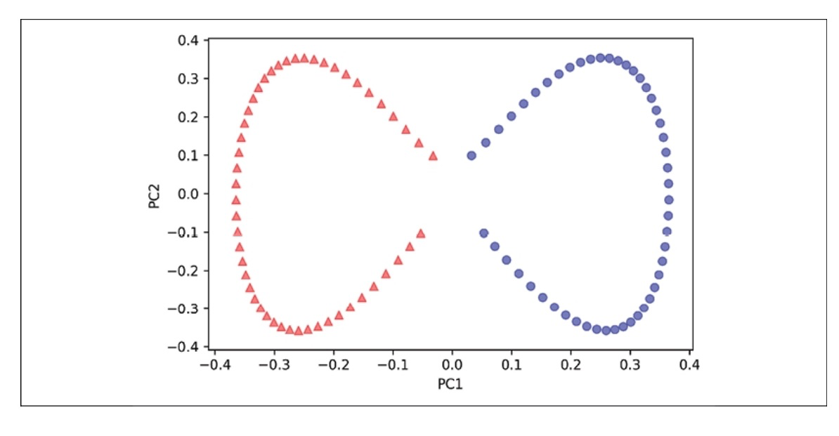
It’s time to generate a new half-moon dataset and then map it onto a one-dimensional subspace using the updated RBF KPCA implementation.

X, y = make_moons(n_samples=100, random_state=123)
alphas, lambdas = rbf_kernel_pca(X, gamma=15, n_components=1)

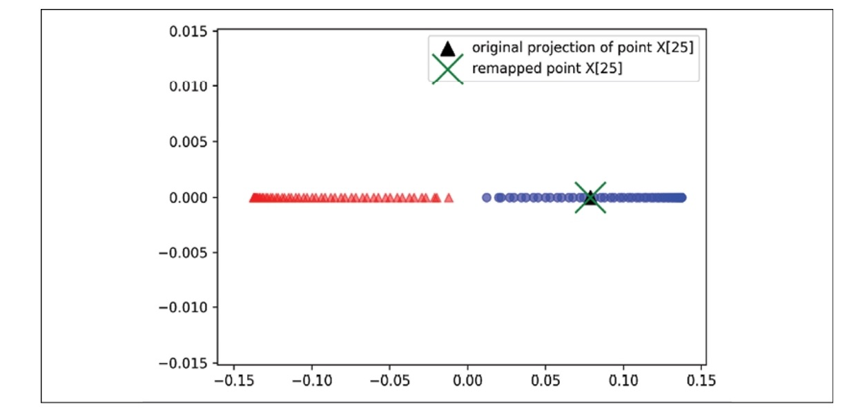
To make sure that we implemented the code for projecting new examples, let’s assume that the 26th point from the half-moon dataset is a new data point, $x’$, and our task is to project it onto this new subspace.

x_new = X[25]
x_proj = alphas[25] # original projection

def project_x(x_new, X, gamma, alphas, lambdas):
  	pair_dist = np.array([np.sum((x_new-row)**2) for now in X])
    k = np.exp(-gamma * pair_dist)
    return k.dot(alpha / lambdas)

The following code has us recreate the initial projection. With the project_x function, we can also project any new data example. Here’s the code:

x_reproj = project_x(x_new, X, gamma=15, alphas=alphas, lambdas=lambdas)

In the scatterplot below, we successfully mapped the example $x’$ onto the first principal component.

Implementing in scikit-learn

Scikit-learn implements a KPCA class in the sklearn.decomposition submodule. The usage is similar to the standard PCA class, and we can specify the kernel via the kernel parameter.

from sklearn.decomposition import KernelPCA
X, y = make_moons(n_samples=100, random_state=123)
scikit_kpca = KernelPCA(n_components=2, kernel='rbf', gamma=15)
X_skernpca = scikit_kpca.fit_transform(X)

Using the code above, we will observe the result plot as below.