
Day57 ML Review - Cross Validation (2)
Bias & Variance, and Learning & Validation Curves
Bias and Variance
Explanations from: "Bias vs. Variance", Strictly By The Numbers. [Online]. Available: https://www.strictlybythenumbers.com/bias-vs-variance. [Accessed: 26-Aug-2024].What is Bias?
Algorithmic bias, or bias in an ML model, occurs when the model overemphasizes certain features. This results in a complex model because the model attempts to generalize the data.
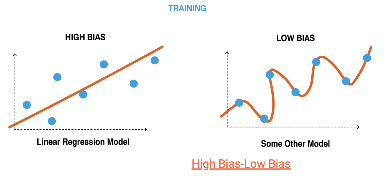
The accuracy of our model is determined by analyzing the disparity between its average prediction and the actual value.
When a model exhibits high bias, it oversimplifies the data, reducing accuracy in both training and test datasets.
Conversely, a low-bias model indicates that it has not captured enough information about the target feature, resulting in inaccuracies due to bias error.
- Error due to bias: Calculated as the most frequently observed difference between the expected prediction of our model and the correct value. (=ground truth)
What is Variance?
As a measure of variability, variance helps us understand how far apart a set of numbers is from its average value.
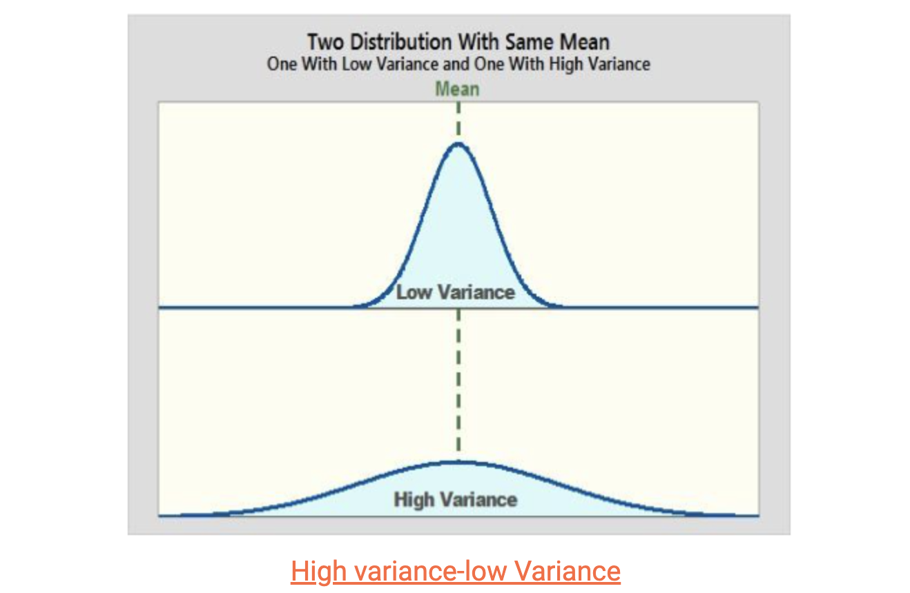
The variance of a machine learning model refers to the variability of the model's predictions for a specific data point, showing how spread out the data is.
High variance suggests that the model is overfitting and cannot generalize to new, unseen data. While it may perform well on the training data, it will likely have significant inaccuracies due to variance error when applied to new data.
On the other hand, low variance means that the predicted values align closely with the actual data, resulting in minor prediction errors.
- Error due to variance: The variance shows how much the predictions for a given point vary between different realizations of the model [=expected variance for the predictions in different realizations of the model]
How are bias and variance related?
The relationship between bias and variance can be described as inverse. When bias is high, variance tends to be low, and vice versa. Striking a balance between low bias and low variance in a model can be complex.
A model with low variance and high bias is advantageous as it lowers the risk of making inaccurate predictions. However, additional support may be required to generalize the dataset properly.
Conversely, a model with low bias and high variance can effectively generalize the dataset, but it may result in inaccurate predictions, ultimately adding complexity to the model.
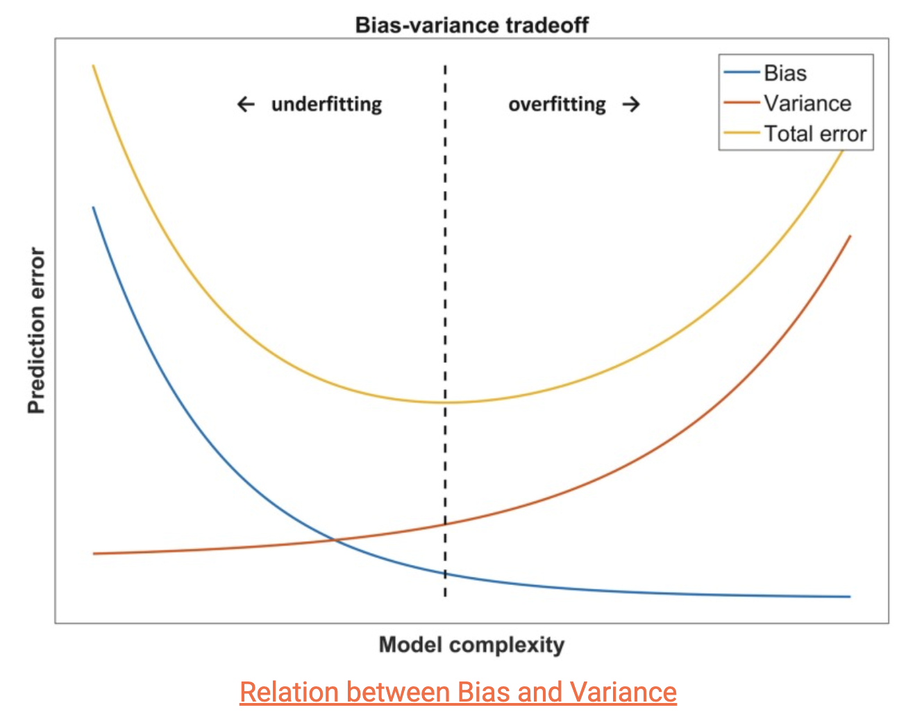
Looking at the graph above, it’s evident that when there is high bias, the model complexity is very low, but the error is very high, which affects the model's predictions. On the other hand, when there is low bias and high variance, the error is also high, making the model inaccurate. In both cases, the training set needs to be generalized better.
We must balance bias and variance to achieve a less complex model with low bias. This trade-off should result in an optimized model complexity and minimized error. There are various methods to achieve this balance, which we will discuss in the following section.
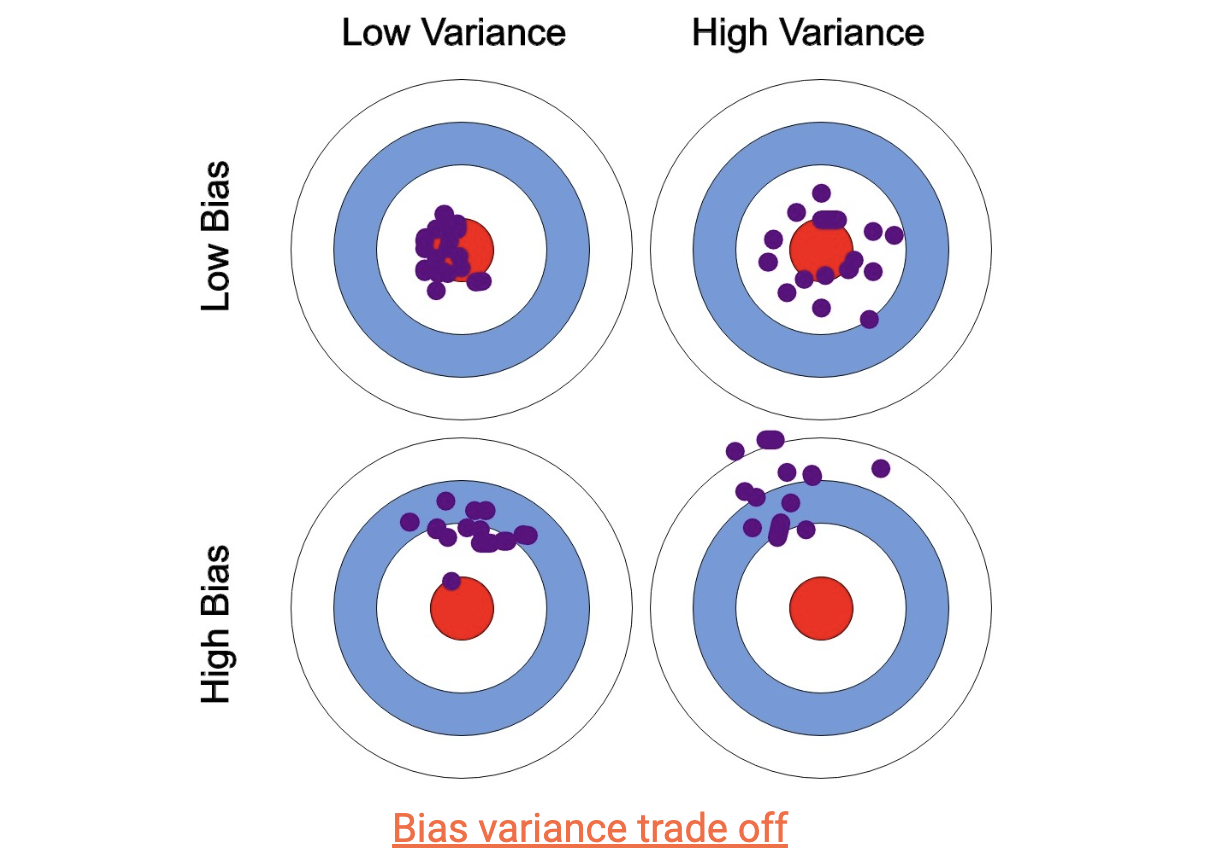
In the graph above, we can observe the predictions and actual values for different scenarios of bias and variance. The optimal scenario is low bias and variance, but achieving this is impractical.
A scenario with high variance and low bias is better than others, indicating a closer match between actual and predicted values. There are several ways to address this bias-variance trade-off.
One approach is to increase the model’s complexity, which decreases bias and increases variance. However, maintaining an acceptable level of variance allows for good accuracy on the training data and minimizes total error, which is the sum of variance error and bias error.
Another method is to expand the training dataset to address overfitting. This also enables an increase in model complexity with minimal variance errors.
However, expanding the training dataset may need to be improved for low-bias models or underfitting situations. Therefore, this method should only be applied in high-variance scenarios.
Summary
Bias is an error that occurs when a machine-learning model makes wrong assumptions. A high bias indicates a large gap between the actual data distribution and the model’s prediction data distribution. If the bias is too high, the model is likely to underfit.
Variance is the error that occurs due to fluctuations in the training data. In other words, if the training data has significant variations and doesn’t follow a consistent pattern, a model well-trained on the data won’t predict new data accurately. This is known as overfitting, which is more likely to happen when the variance is high.
The bias-variance trade-off describes a relationship in which improving bias and variance in a model simultaneously is challenging. Therefore, it’s essential to consider both factors when choosing a model.
- This is true for simpler models when the bias is significant, and the variance is slight. In this case, there is a substantial difference between the data distribution and the model that fits it. However, even if the training data changes, the resulting model remains similar in shape.
- On the other hand, when the bias is slight and the variance is significant, it’s more common in complex models. Here, the difference between the data distribution and the corresponding model is subtle, yet the shape of the resulting models varies as the training data changes.
Learning Curves
By analyzing learning and validation curves, we can assess and diagnose the model and enhance the performance of a learning algorithm. Learning curves are instrumental in determining whether a learning algorithm suffers from overfitting (high variance) or underfitting (high bias). Additionally, the insights provided by validation curves enable us to effectively address and rectify common issues encountered by a learning algorithm.
Using the code below, we will observe whether those models are overfitted or underfitted.
import matplotlib.pyplot as plt
from sklearn.model_selection import learning_curve
pipe_lr = make_pipeline(StandardScaler(),
                       LogisticRegression(penealty='12', random_state=1, solver='lbfgs', max_iter=10000))
train_sizes, train_scores, test_scores = \
learning_curve(estimator=pipe_lr,
               X=X_train,
               y=y_train,
               train_sizes = np.linspace(0.1, 1.0, 10),
               cv=10,
               n_jobs=1)

train_mean = np.mean(train_scores, axis=1)
train_std = np.std(train_scores, axis=1)
test_mean = np.mean(test_scores, axis=1)
test_std = np.std(test_scores, axis=1)
plt.plot(train_sizes, train_mean, color='blue', marker='o', markersize=5, label='Training Accuracy')
plt.fill_between(train_sizes, test_mean + test_std, test_mean - test_std, alpha=0.15, color='green')
plt.grid()
plt.xlabel('Number of training examples')
plt.ylabel('Accuracy')
plt.legend(loc='lower right')
plt.ylim([0.8, 1.03])
plt.show()
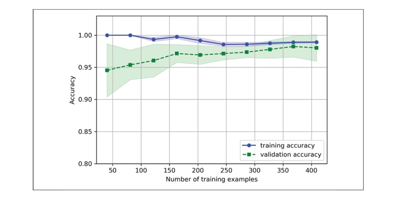
We included max_iter=10000 as an extra parameter when creating the LogisticRegression object (which defaults to 1,000 iterations) to prevent convergence problems for smaller datasets or very high regularization parameter values. The code above generates the data plot chart shown below.
When using the learning_curve function, we can utilize the train_size parameter to precisely control the absolute or relative number of training examples employed in generating the learning curves. In this instance, we have defined train_sizes=np.linspace(0.1, 1.0, 10) to enable the use of 10 evenly distributed relative intervals for the training dataset sizes. By default, the learning_curve function leverages stratified k-fold cross-validation to compute a classifier's cross-validation accuracy. In our case, we specify k=10 using the `cv` parameter to achieve 10-fold stratified cross-validation.
Next, we computed the mean accuracies using the cross-validated training and test scores for various training dataset sizes.
Our model excels on training and validation datasets in the previous learning curve plot when trained on more than 250 examples. Additionally, we notice that the training accuracy improves for datasets with fewer than 250 examples, and the difference between validation and training accuracy increases, signifying a higher level of overfitting.
Validation Curves
Validation curves are related to learning curves, but instead of plotting the training and test accuracies as sample size functions, we vary the values of the model parameters, for example, the inverse regularization parameter, C, in logistic regression.
from sklearn.model_selection import validation_curve
param_range = [0.001, 0.01, 0.1, 1.0, 10.0, 100.0]
train_scores, test_scores = valdition_curve(estimator=pipe_lr,
                                           X=X_train,
                                           y=y_train,
                                           param_name='logisticregression_C',
                                           param_range=param_range,
                                           cv=10)
train_mean = np.mean(train_scores, axis=1)
train_std = np.std(train_scores, axis=1)
test_mean = np.mean(test_scores, axis=1)
test_std = np.std(test_scores, axis=1)
Like the learning_curve function, the validation_curve function utilizes stratified k-fold cross-validation as the default method for estimating the classifier’s performance. Within the validation_curve function, we specified the parameter to be evaluated, the inverse regularization parameter `C` of the `LogisticRegression` classifier. We accessed the LogisticRegression object inside the scikit-learn pipeline and specified a value range using the param_range parameter. Like the previous section’s learning curve example, we created a plot displaying the average training and cross-validation accuracies and their corresponding standard deviations.
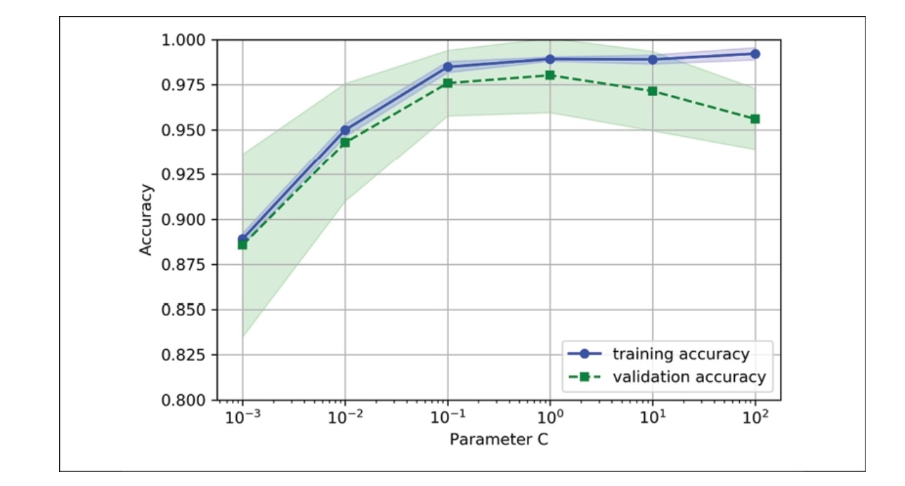
When the regularization strength is increased (small values of C), the model slightly underfits the data. Conversely, when we have large values of C, meaning reduced regularization strength, the model tends to overfit the data slightly. In this scenario, the optimal range for the C value is between 0.01 and 0.1.
Leave a comment