Day58 ML Review - Cross Validation (3)

📚 The Start of Recording TIL Summer ‘24 : Why Did I Start This Project? 🚀

🔔 Don't Miss: Continous Records of TIL '25 (Still On-Going!) 🌟

✨ A New Chapter in TIL '25: Reflecting, Growing, and Moving Forward 📖

Grid Search for Fine-Tuning Machine Learning Models

Grid Search

Grid search is a method for fine-tuning the hyperparameters of machine learning models. It involves defining a grid of hyperparameter values and systematically searching through the grid to find the combination of parameters that results in the best model performance, as determined by a specific metric.

How it works

1. Define the Parameters: We start by defining a list or grid of values for various hyperparameters we want to tune. This might include parameters like learning rate, number of hidden layers, number of trees in a decision forest, etc.
2. Cross-Validation Setup: Grid search is often used in conjunction with cross-validation to ensure that the tuning process does not overfit to a particular subset of the data. In $k$-fold cross-validation, the training set is split into $k$ smaller sets (or folds). The model is trained on $k-1$ of these folds, with the remaining part used as a pseudo-test set to compute a performance measure such as accuracy, F1 score, etc.
3. Exhaustive Search: The method then systematically trains models using every combination of parameters in your grid and evaluates each model using cross-validation. For each combination, the average score across all folds is computed.
4. Select Best Parameters: Once all combinations have been evaluated, the grid search selects the best parameter combination in the cross-validation process.
5. Final Model: A final model is often trained on the entire training set using the best parameter settings.

This method is exhaustive but can also be computationally expensive, especially with large datasets, a wide range of parameter values, or many parameters to tune. As an alternative, methods like random search or Bayesian optimization provide faster but less exhaustive approaches to hyperparameter tuning.

from sklearn.model_selection import GridSearchCV
from sklearn.svm import SVC
pipe_svc = make_pipeline(StandardScaler(), SVC(random_state=1))
param_range = [0.0001, 0.001, 0.01, 0.1, 1.0, 10.0, 100.0, 1000.0]
param_grid = [{'svc__C': param_range,
              'svc__kernel': ['linear']},
             {'svc__C': param_range,
             'svc__gamma': param_range,
             'svc__kernel': ['rbf']}]
gs = GridSearchCV(estimator=pipe_svc,
                 param_grid=param_grid,
                 scoring='accuracy',
                 cv=10,
                 refit=True,
                 n_jobs=-1)
gs = gs.fit(X_train, y_train)
print(gs.best_score)
print(gs.best_params_)

In the previous code, we used the GridSearchCV object from the sklearn.model_selection module to train and optimize an SVM pipeline. We specified the parameters we wanted to tune by setting the param_grid parameter of GridSearchCV to a list of dictionaries. For the linear SVM, we only focused on tuning the inverse regularization parameter, C, while for the RBF kernel SVM, we tuned both the svc __C and svc__gammaparameters. It’s important to note that the svc__gamma parameter is specific to kernel SVMs.

We found the score of the best-performing model using the best_score_ attribute and examined its parameters using the best_params_ attribute. In this instance, the RBF kernel SVM model with svc__C = 100.0 achieved the highest $k$-fold cross-validation accuracy of 98.5%.

Side Note: Nested Cross-Validation

Another recommendation for hyperparameter tuning is nested cross-validation. This method involves two layers of cross-validation: an outer loop and an inner loop. The purpose is to ensure that the model evaluation is as unbiased as possible, particularly in scenarios involving hyperparameter tuning.

We use an outer k-fold cross-validation loop to split the data into training and test folds. Within this, there is an inner loop that selects the model using k-fold cross-validation on the training fold.

Once the model is selected, the test fold is used to evaluate the model’s performance. The diagram below illustrates the concept of nested cross-validation. This approach is particularly useful for large datasets where computational performance is crucial.

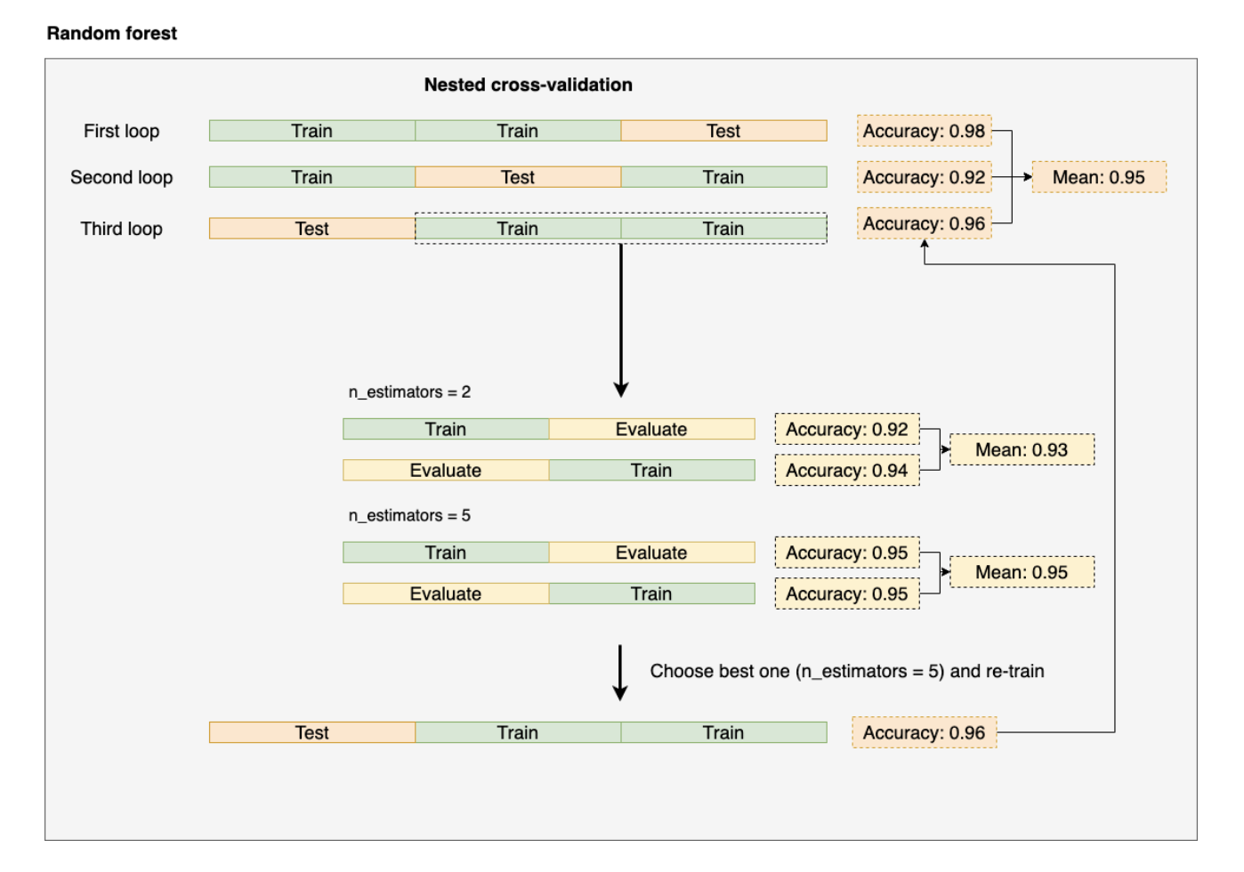
(Image from: https://ploomber.io/blog/nested-cv/)

In Scikit-learn, we can employ the code as follows.

gs = GridSearchCV(estimator=pipe_svc,
                  param_grid=param_grid,
                  scoring='accuracy',
                  cv=2)
scores = cross_val_score(gs, X_train, y_train, scoring='accuracy', cv=5)
print('CV accuracy: %.3f +/- %.3f' % (np.mean(scores), np.std(scores)))

From the code above, we can see that CV accuracy is 0.974.

The average cross-validation accuracy that we obtain provides a reliable estimate of the model’s performance when its hyperparameters are fine-tuned and used on new data.

For instance, we can employ a nested cross-validation technique to compare an SVM model with an essential decision tree classifier. We will focus solely on adjusting the decision tree’s depth parameter to simplify the comparison.

from sklearn.tree import DecisionTreeClassifier
gs = GridSearchCV(estimator=DecisionTreeclassifier(random_state=0),
                  param_grid=[{'max_depth': [1,2,3,4,5,6,7,None]}],
                  scoring='accuracy'
                  cv=2)
scores = cross_val_scores(gs, X_train, y_train,scoring='accuracy', cv=5)
print('CV accuracy: %.3f +/- %.3f' % (np.mean(scores), np.std(scores)))

We could get the result of CV accuracy of 0.934.

Based on the provided codes, the SVM model achieved a nested cross-validation performance of 97.4%, which is significantly higher than the decision tree’s performance of 93.4%. Therefore, it is expected that the SVM model would be the better choice for classifying new data from the same population as this dataset.