
Day59 ML Review - Cross Validation (4)
Confusion Matrix and F1 score

Confusion Matrix
Image and Explanation from Evidently AI Webpage(https://www.evidentlyai.com/classification-metrics/confusion-matrix)
A confusion matrix is simply a square matrix that reports the count of the true positive(TP), true negative(TN), false positive(FP), and false negative(FN) predictions of the classifier, as shown below.
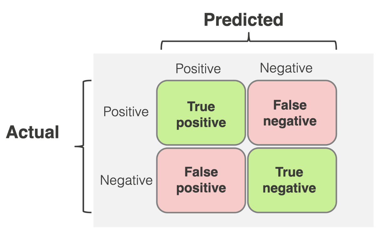
The confusion matrix displays the number of correct and false predictions. However, absolute numbers may only sometimes be practical. We also need relative metrics to compare models or track their performance over time. You can derive such quality metrics directly from the confusion matrix.
Error and Accuracy
Both the prediction error (ERR) and accuracy (ACC) offer general insight into the misclassification of examples. The error represents the sum of all false predictions divided by the total number of predictions.
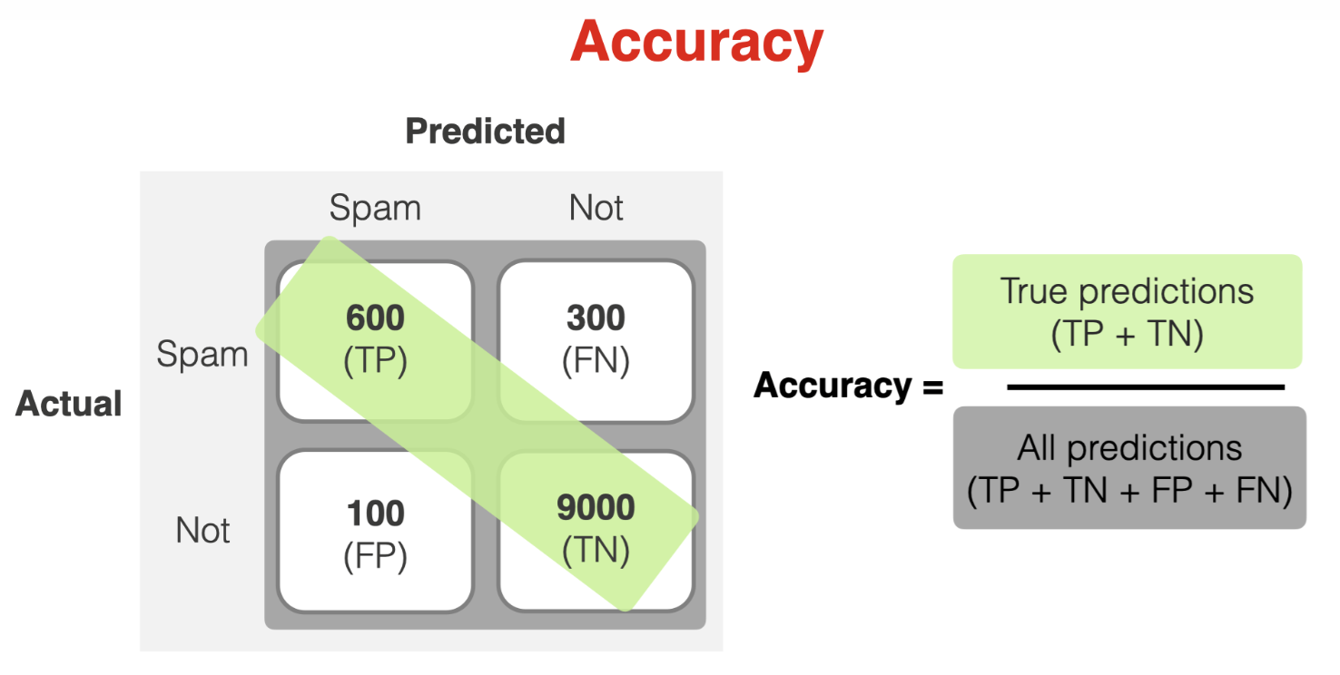
Accuracy refers to the proportion of all correct classifications, regardless of whether they are positive or negative. It is mathematically defined as:
Also, we can calculate directly from the error.
However, accuracy can be misleading for imbalanced datasets when one class has significantly more samples. For example, let’s assume we have many non-spam emails: 9100 out of 10000 are regular emails. The overall model 'correctness' is heavily skewed to reflect how well the model can identify those non-spam emails. The accuracy number could be more informative if we are interested in catching spam.
Recall and Precision
The true positive rate (TPR) and false positive rate (FPR) are performance metrics, beneficial for imbalanced class problems.
$TPR=\frac{TP}{P}=\frac{TP}{FN+TP}$
Recall shows the model’s share of true positive predictions out of all positive samples in the dataset. In other words, recall shows how many instances of the target class the model can find.
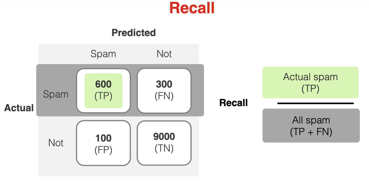
Recall is a helpful metric when the cost of false negatives is high. For example, we can optimize for recall if we do not want to miss any spam (even at the expense of falsely flagging some legitimate emails).
Precision is the share of true positive predictions in all positive predictions. In other words, it shows how often the model is suitable when it predicts the target class.
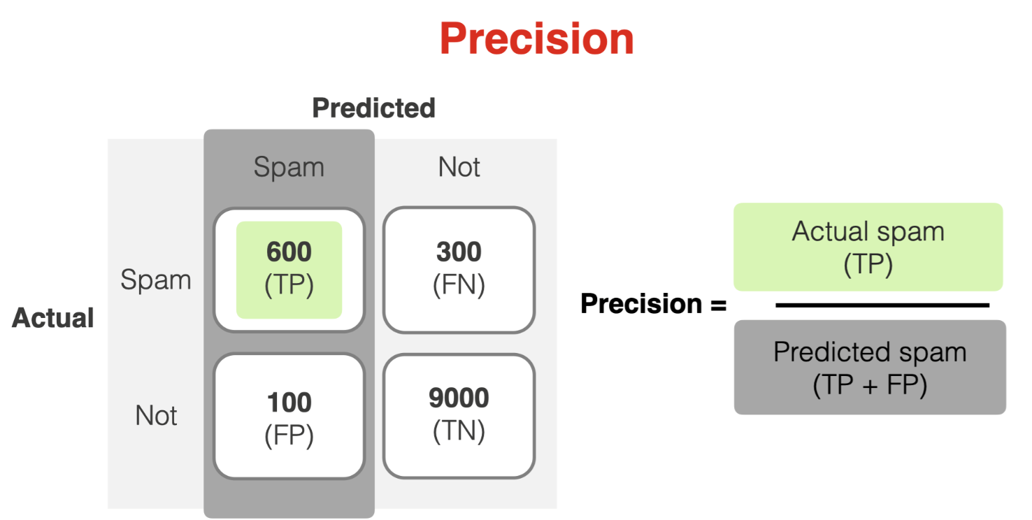
Precision is an important metric when the cost of false positives is high. If we want to avoid sending good emails to spam folders, we should focus on precision.
The performance metrics precision (PRE) and recall (REC) are related to those TP and TN rates, and in fact, REC is synonymous with TPR:
F1 Score
Image and Explanation from Google Developer_ML Concepts Webpage( https://developers.google.com/machine-learning/crash-course/classification/accuracy-precision-recall)
In machine learning, the F1 score, also known as the F-measure, is a performance metric that measures a model’s accuracy by combining its precision and recall scores into a single value. The F1 score is calculated using the harmonic mean of the precision and recall scores, which encourages similar values for both. The F1 score ranges from 0–100%, with higher scores indicating better quality classifiers.
Balancing the trade-offs between precision (PRE) and recall (REC) is essential in many applications. Precision and recall are often used to strike a balance between the two, resulting in the so-called F1 score.
Those scoring metrics are all implemented in scikit-learn and can be imported from the sklearn.metrics module, as shown in the following code snippet.
from sklearn.metrics import precision_score
from sklearn.metrics import recall_score, f1_score
print('Precision: %.3f' % precision_score(y_true=y_test, y_pred=y_pred))
print('Recall: %.3f' % recall_score(y_true=y_test, y_pred=y_pred))
print('F1: %.3f' % f1_score(y_true=y_test, y_pred=y_pred))
Using the scoring parameter as demonstrated below, we can employ an alternative scoring metric instead of accuracy in the GridSearchCV.
from sklearn.metrics import make_scorer, f1_score
c_gamma_range = [0.01, 0.1, 1.0, 10.0]
param_grid = [{'svc__C': c_gamma_range,
              'svc__kernel': ['linear']},
             {'svc__C': c_gamma_range,
             'svc__gamma': c_gamma_range,
             'svc__kernel': ['rbf']}]
scorer = make_scorer(f1_score, pos_label=0)
gs = GridSearchCV(estimator=pipe_svc,
                 param_grid=param_grid,
                 scoring=scorer,
                 cv=10)
gs = gs.fit(X_train, y_train)
print(gs.best_score_)
print(gs.best_params_)
Choice of Metrics and Tradeoffs
Table from: https://developers.google.com/machine-learning/crash-course/classification/accuracy-precision-recall| Metric | Guidance |
|---|---|
| Accuracy | Use as a rough indicator of model training progress/convergence for balanced datasets.For model performance, use only in combination with other metrics.Avoid for imbalanced datasets. Consider using another metric. |
| Recall (True positive rate) | Use when false negatives are more expensive than false positives. |
| False positive rate | Use when false positives are more expensive than false negatives. |
| Precision | Use when it’s very important for positive predictions to be accurate. |
Scikit-learn Applications
Scikit-learn provides a convenient confusion_matrix function that we can use, as follows.
from sklearn.metrics import confusion_matrix
pipe_svc.fit(X_train, y_train)
y_pred = pipe_svc.predict(X_test)
confmat = confusion_matrix(y_true=y_test, y_pred=y_pred)
print(confmat)
After executing the code, the array returned provides information about the different types of errors the classifier made on the test dataset. Using Matplotlib’s matshow function, we can map this information onto the confusion matrix illustration in the figure below.
fig, ax = plt.subplots(figsize=(2.5, 2.5))
ax.matshow(confmat, cmap=plt.cm.Blues, alpha=0.3)
for i in range(confmat.shape[0]):
              for j in range(confmat.shpae[1]):
              ax.text(x=j, y-1, s=confmat[i, j],
                     va='center', ha='center')
plt.xlabel('Predicted label')
plt.ylabel('True label')
plt.show()
Leave a comment