Day06 ML Review - Principle Component Analysis (2)

📚 The Start of Recording TIL Summer ‘24 : Why Did I Start This Project? 🚀

🔔 Don't Miss: Continous Records of TIL '25 (Still On-Going!) 🌟

✨ A New Chapter in TIL '25: Reflecting, Growing, and Moving Forward 📖

Applications on Machine Learning & Further Explanations

All explanation is mainly from: (https://ddongwon.tistory.com/114)

Let’s assume we have a dataset of 5 points representing weight and height. Here’s how Principal Component Analysis (PCA) can be applied:

1) Centering the Data

First, calculate the average (mean) values for each dimension: weight (x-axis) and height (y-axis). Then, shift all data points to align these mean values with the origin. This involves subtracting the mean of each variable from their respective values, resulting in a new dataset centered around the origin. This step is crucial, as it normalizes the data by removing any inherent bias towards a particular scale or starting point.

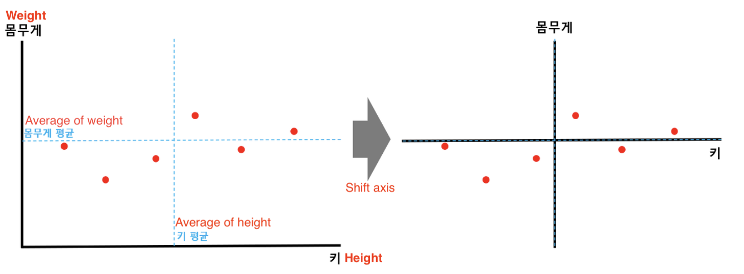
The graph shows the original data points and their averages on each axis. After centering, the intersection of these average values becomes the graph’s origin.

2) Finding the Principal Component

Once the data is centered, the next goal is to draw a line through the origin (0,0) and find the direction along which the **data's variance is maximized.** This is done by rotating a hypothetical line around the origin and calculating the sum of the squares of the perpendicular distances (projected points) from the data points to the line.

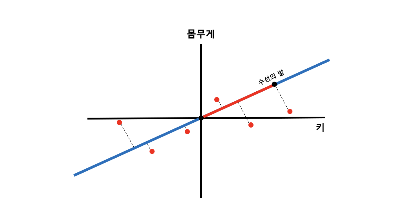
• Mathematical Objectives: In Principal Component Analysis (PCA), the goal is to maximize the sum of squares of the distances, as these distances indicate the variance of the data when it's projected onto a line. The direction where this sum of squared distances is maximized represents the first principal component, PC1.

3) Identifying the First Principal Component (PC1)

The line that maximizes the sum of squares becomes the first principal component. The vector that defines this line is the "eigenvector" associated with the largest eigenvalue since it accounts for the most variance among all possible line orientations.

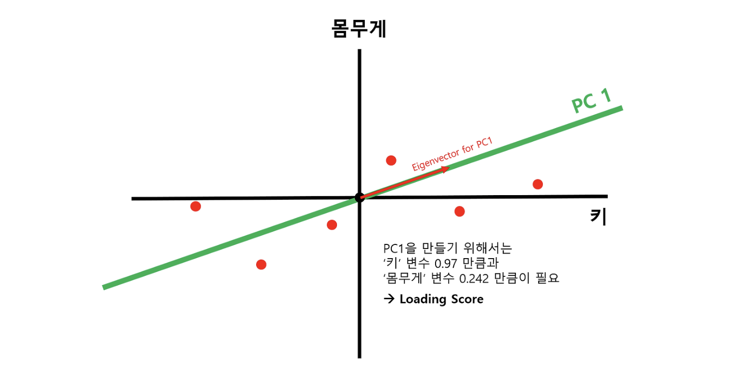
• Loading Score The Loading scores are the coordinates of the eigenvector (also referred to as the components of the eigenvector) and indicate the contribution of each original variable (weight and height in this case) to the principal component. In this example, a loading score ratio of 0.97 for x (weight) and 0.242 for y (height) indicates how much weight each variable has in the principal component.

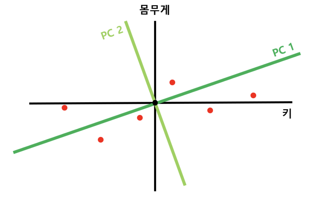
4) Identifying the Second Principal Component (PC2)

Once PC1 is established, the next step is to find a direction that is orthogonal (perpendicular) to PC1 to identify the second principal component (PC2). This step is crucial for ensuring the new features are uncorrelated, a key aspect of PCA.

• In 2D Scenarios: Only one line is orthogonal to PC1 for two-dimensional data. This line is automatically the second principal component.

• In Higher Dimensions: The set of directions orthogonal to PC1 forms a hyperplane for data with more than two dimensions. The next principal component (PC2) is the direction within this hyperplane that maximizes the variance of the data projected onto it, similar to how PC1 was determined.

• Generalization to N Dimensions: PCA identifies N orthogonal principal components in an N-dimensional space, each capturing different aspects of the data’s variance, following the steps for PC1 and PC2.

5) Rotation to Principal Component Axes and Scree Plot Creation

After identifying the principal components, we can transform the data by rotating it such that the axes align with these components. This reorientation simplifies the interpretation of the data by aligning it along the axes of maximum variance.

• Data Transformation: Rotate the dataset so that PC1 and PC2 are aligned with the x-axis and y-axis, respectively. This rotation transforms the dataset into a new coordinate system defined by the principal components.
• Scree Plot: A scree plot is then used to visualize the proportion of the total variance captured by each principal component. It plots the eigenvalues or the sum of squares values associated with each principal component. The SS values indicate how much variance each principal component captures from the data.
• Example Calculation: The SS ratio of PC1 to PC2 is 8.9:1.1, indicating that PC1 accounts for approximately 89% of the total variance, while PC2 accounts for about 11%. This visualization is helpful for deciding how many principal components to retain based on their contribution to the total variance.
• Dimensionality Reduction Decision: If the first principal component (PC1) captures a significant amount of the total variance, for example, 89%, you might decide to simplify the dataset by keeping only PC1. This simplification helps to reduce the complexity of the data representation while retaining as much variance as possible, which is the main objective of PCA - to reduce dimensionality while preserving as much information as possible.