Day64 ML Review - Ensemble Method (3)

📚 The Start of Recording TIL Summer ‘24 : Why Did I Start This Project? 🚀

🔔 Don't Miss: Continous Records of TIL '25 (Still On-Going!) 🌟

✨ A New Chapter in TIL '25: Reflecting, Growing, and Moving Forward 📖

Using the Majority Voting Principle to Make Predictions, and Evaluating & Tuning the Ensemble Classifier

We will continue to train three different classifiers to predict and compare the results.

• Logistic Regression Classifier
• Decision Tree Classifier
• K-nearest Neighbors Classifier

We will then evaluate the model performance of each classifier via 10-fold cross-validation on the training dataset before we combine them into an ensemble classifier.

>>> from sklearn.model_selection import cross_val_score
>>> from sklearn.linear_model import LogisticRegression
>>> from sklearn.tree import DecisionTreeClassifier
>>> from sklearn.neighbors import KNeighborsClassifier
>>> from sklearn.pipeline import Pipeline
>>> import numpy as np

>>> clf1 = LogisicRegression(penalty='l2', C=0.001, solver='lbfgs', random_state=1)
>>> clf2 = DecisionTreeClassifier(max_depth=1, creterion='entropy', random_state=0)
>>> clf3 = KNeighborsClassifier(n_neighbors=1, p=2, metric='minkowski')

1. Parameters for Logistic Regression(clf1)

• penalty=L2: This parameter specifies the type of regularization applied to the model:
  • 'l1': Lasso regularization (forces some coefficients to be exactly zero, which can be used for feature selection).
  • 'l2': Ridge regularization (shrinks coefficients but keeps them non-zero).
  • 'elasticnet': Combination of L1 and L2 regularization.
  • 'none': No regularization.

• C=0.001: This is the inverse of the regularization strength (i.e., 1/λ where λ is the regularization parameter). A smaller value of C implies more robust regularization. In this case, C=0.001 means high regularization.

• solver='lbfgs': The algorithm used to solve the optimization problem. lbfgs stands for “Limited-memory Broyden–Fletcher–Goldfarb–Shanno,” a quasi-Newton method. It’s efficient for small to medium datasets and supports L2 regularization.

Side note: Different types of ‘solver’

• Use lbfgs for most cases, especially when dealing with multi-class classification or medium-sized datasets.

• Use liblinear when we have large datasets dealing with binary classification or sparse data.
• Use sag or saga when we have massive datasets. Choose saga if we need L1 or elastic net regularization.
• Use newton-cg when dealing with multi-class classification and need a reliable but slower alternative to lbfgs.

2. Decision Tree(clf2)

• max_depth=1: The maximum depth of the tree. Limiting the depth of the tree to 1 means that it will only be able to split once, resulting in a decision stump (i.e., a very shallow tree that essentially only creates one decision).

• criterion='entropy': This parameter defines the function to measure the quality of a split:

  • 'gini': The Gini impurity (default).
  • 'entropy': The information gain (based on information theory) is used to choose the split points. Using 'entropy' means the algorithm will calculate the information gain at each split.

3. KNeighborsClassifier (clf3)

• n_neighbors=1: This specifies the number of neighbors to consider when making a classification decision. Setting n_neighbors=1 means the classifier will look at the closest neighbor (1-NN).

• p=2: This is the power parameter for the Minkowski distance metric. When p=2, the Minkowski distance becomes equivalent to the Euclidean distance (L2 norm). If p=1, it becomes the Manhattan distance (L1 norm).

• metric='minkowski': This parameter defines the distance metric used to calculate the “closeness” of data points. The default is 'minkowski', which encompasses both Euclidean and Manhattan distances based on the value of p. With p=2, the metric will calculate the Euclidean distance.

Continuing with the above code-

>>> from sklearn.model_selection import cross_val_score
>>> from sklearn.linear_model import LogisticRegression
>>> from sklearn.tree import DecisionTreeClassifier
>>> from sklearn.neighbors import KNeighborsClassifier
>>> from sklearn.pipeline import Pipeline
>>> import numpy as np

>>> clf1 = LogisicRegression(penalty='l2', C=0.001, solver='lbfgs', random_state=1)
>>> clf2 = DecisionTreeClassifier(max_depth=1, creterion='entropy', random_state=0)
>>> clf3 = KNeighborsClassifier(n_neighbors=1, p=2, metric='minkowski')


>>> pipe1 = Pipeline([['sc', StandardScaler()], ['clf', clf1]])
>>> pipe3 = Pipeline([['sc', StandardScaler()], ['clf', clf3]])

>>> clf_labels = ['Logistic Regression', 'Decision Tree', 'KNN']
>>> print('10-fold cross validation: \n')
>>> for clf, label in zip([pipe1, clf2, pipe3], clf_labels):
      scores = cross_val_score(estimator=clf, X=X_train, y=y_train, cv=10,
                              scoring='roc_auc')
      print("ROC AUC: %0.2f (+/- %0.2f [%s])"
           % (scores.mean(), score.std(), label))

The result will be received as follows.

10-fold cross validation
ROC AUC : 0.92 (+/- 0.15) [Logistic Regression]
ROC AUC : 0.87 (+/- 0.18) [Decision Tree]
ROC AUC : 0.85 (+/- 0.13) [KNN]

The Logistic Regression and KNN algorithms are not scale-invariant, in contrast to decision trees, so we made up a pipeline for stndardizing the variables.

Then, let’s combine the individual classifiers for majority rule voting in our MajorityVoteClassifier:

>>> mv_clf = MajorityVoteClassifier(clssifiers=[pipe1, clf2, pipe3])
>>> clf_labels += ['Majority Voting']
>>> all_clf = [pipe1, clf2, pipe3, mv_clf]
>>> for clf, label in zip(all_clf, clf_labels):
  	scores = cross_val_score(estimator=clf, X=X_train, y=y_train, cv=10, scoring='roc_auc')
  	print("ROC AUC: %0.2f (+/- %0.2f) [%s]") % (scores.mean(), scores.std(), label)

ROC AUC: 0.92 (+/- 0.15) [Logistic Regression]
ROC AUC: 0.87 (+/- 0.18) [Decision Tree]
ROC AUC: 0.85 (+/- 0.13) [KNN]
ROC AUC: 0.98 (+/- 0.05) [Majority Voting]

As we can observe and compare the results from the code above, the performance of MajorityVotingClassifier has improved over the individual classifiers in the 10-fold cross-validation evaluation.

Evaluating and Tuning the Ensemble Classifier

We will further compute the ROC curves from the test dataset to check that MajorityVoteClassifier generalizes well with the unseen data.

>>> from sklearn.metrics import roc_curve
>>> from sklearn.metrics import auc
>>> colors = ['black', 'orange', 'blue', ;green]
>>> linestyles = [':', "--", "-.", "-"]
>>> for clf, label, clr, ls in zip(all_clf, clf_labels, colors, line_styles):
  
    	# Assuming the label of the positive class is 1
    		y_pred = clf.fit(X_train, y_train).predict_proba(X_test)[:, 1]
    
    		fpr, tpr, thresholds = roc_curve(y_true=y_test, y_score=y_pred)
    		roc_auc = auc(x=fpr, y=tpr)    
    		plt.plot(fpr, tpr, 
        		     color=clr,
            		 linestyle=ls,
		             label='%s (AUC = %0.2f)' % (label, roc_auc))

>>> plt.legend(loc='lower right')
>>> plt.plot([0,1], [0,1], linestyle='--', color='gray', linewidth=2)
>>> plt.xlim([-0.1, 1.1])
>>> plt.ylim([-0.1, 1.1])
>>> plt.grid(alpha=0.5)
>>> plt.xlabel('False Postive Rate (FPR)')
>>> plt.ylabel('True Postive Rate (TPR)')
>>> plt.show()

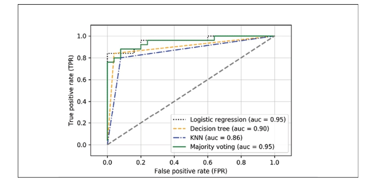
Upon reviewing the ROC plot, it’s evident that the ensemble classifier has demonstrated strong performance on the test dataset with an ROC AUC of 0.95. Interestingly, the logistic regression classifier also exhibits similar strong performance on the same dataset. This could be attributed to the dataset’s small size, leading to high variance, particularly in terms of how the dataset was split.

The best cross-validation results are achieved when we opt for a lower regularization strength (C=0.001). Surprisingly, the tree depth does not seem to have an impact on the model performance, indicating that a decision stump might be adequate for separating the data. It’s crucial to remember that repeatedly using the test dataset for model evaluation is not advisable. That’s why we use alternative approaches for ensemble learing: bagging & boosting.