
Day65 ML Review - Ensemble Method (4)
Bagging & Boosting : Basic Concepts & Code Implementation

In contrast to using the identical training dataset for fitting each classifier in the ensemble, we utilize bootstrap samples, random samples drawn with replacements from the original training dataset. This approach is why bagging is also referred to as bootstrap aggregating.
Ensemble learning in machine learning integrates several individual models to form a more robust and accurate predictive framework. By utilizing the unique strengths of various models, this approach seeks to reduce errors, boost performance, and strengthen prediction reliability, ultimately enhancing outcomes across different machine learning and data analysis tasks.
Explanations from Scaler and Analytics Vidhya
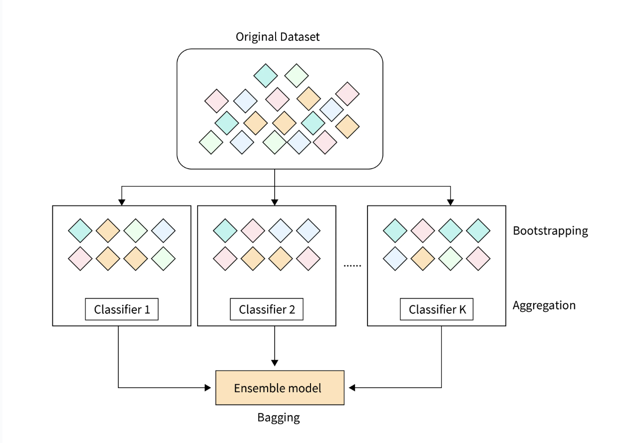
Image from: Scaler Topics "Bagging in Machine Learning"
Bagging (Bootstrap Aggregating)
- Bagging, which stands for Bootstrap Aggregating, is a machine learning ensemble technique used to improve the accuracy and reliability of predictive models. It involves creating multiple subsets of the training data by using random sampling with replacement. These subsets train multiple base learners, such as decision trees, neural networks, or other models.
-
It involves the following steps:
- Data Sampling: Generating several subsets of the training dataset through bootstrap sampling, which involves random sampling with replacement.
- Model Training: Training a separate model on each subset of the data.
- Aggregation: Combining predictions from all models—averaging for regression and using majority voting for classification—to generate the final output.
- Key benefits are the following:
- Reduces Variance: By averaging multiple predictions, bagging minimizes the variance of the model and helps prevent overfitting.
- Improves Accuracy: Combining multiple models usually leads to better performance than individual models.
For example, seven training instances are randomly sampled in each bagging round as below.
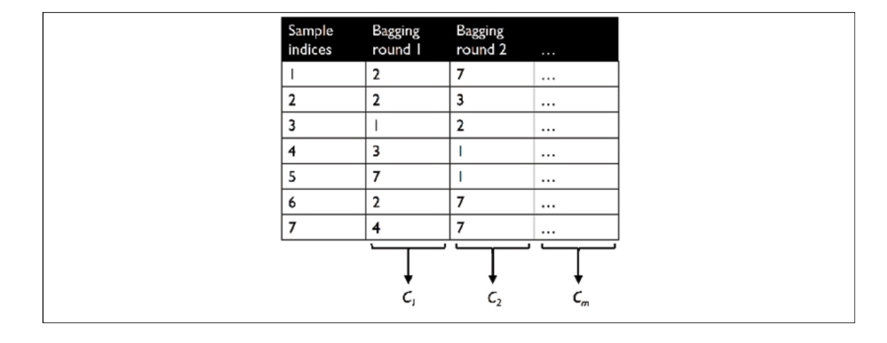
The process entails training a classifier by generating subsets, termed bootstrap samples. Typically, an unpruned decision tree is denoted as $C_j$. In this approach, each classifier is trained on a random subset from the training dataset, labeled as Bagging Round 1, Bagging Round 2, and so forth. It’s important to note that each subset can include duplicate examples, and some original examples might need to be present in the resampled dataset due to the nature of sampling with replacement. After training the individual classifiers on these bootstrap samples, their predictions are aggregated using a majority voting system.
Code Implementation
The scikit-learn library already includes the BaggingClassifier algorithm, which we can import from the ensemble submodule. In this case, we will use an unpruned decision tree as the base classifier and create an ensemble of 500 decision trees trained on different bootstrap samples of the training dataset.
>>> from sklearn.ensemble import BaggingClassifier
>>> tree = DecisionTreeClassifier(criterion='entropy', random_state=1, max_depth=None)
>>> bag = BaggingClassifier(base_estimator=tree, n_estimators=500,
                            max_samples=1.0, max_features=1.0,
                            bootstrap=True, bootstrap_features=False, n_jobs=1, random_state=1)
We will assess the accuracy score of predictions on both the training and test datasets to evaluate how the bagging classifier performs compared to a single unpruned decision tree.
>>> from sklearn.metrics import accuracy_score
>>> tree = tree.fit(X_train, y_train)
>>> y_train_pred = tree.predict(X_train)
>>> y_test_pred = tree.predict(X_test)
>>> tree_train = accuracy_score(y_train, y_train_pred)
>>> tree_test = accuracy_score(y_test, y_test_pred)
>>> print("Decision Tree Train/Test Accuracies %.3f/%.3f" % (tree_train, tree_test))
Decision Tree Train/Test Accuracies 1.000/0.833
The decision tree and bagging classifier achieve 100 percent training accuracy on the training dataset. Nevertheless, the bagging classifier shows marginally improved generalization performance on the test dataset. Next, let’s compare the decision regions of the decision tree and the bagging classifier.
>>> bag = bag.fit(X_train, y_train)
>>> y_train_pred = bag.predict(X_train)
>>> y_test_pred = bag.predict(X_test)
>>> bag_train = accuracy_score(y_train, y_train_pred)
>>> bag_test = accuracy_score(y_test, y_test_pred)
>>> print('Bagging train/test accuracies %.3f/%.3f' % (bag_train, bag_test))
Bagging train/test accuracies 1.000/0.917
While both the decision tree and bagging classifier achieve identical training accuracies (100 percent each) on the training dataset, the bagging classifier demonstrates slightly superior generalization performance when evaluated on the test dataset.
Complex classification tasks and a dataset’s high dimensionality can quickly result in overfitting with single decision trees. This is where the bagging algorithm demonstrates its strengths. However, bagging only effectively reduces model bias, which occurs when models are overly simplistic and fail to capture data trends accurately. Therefore, we aim to implement bagging on a group of low-bias classifiers, such as unpruned decision trees. Then, we will discuss boosting further.
Boosting (adaptive Boosting)
Boosting is another ensemble learning method that aims to create a robust model by combining several weak learners.
-
The process includes these steps:
- Sequential Training: Models are trained one after another, with each aiming to fix the errors of the previous ones.
- Weight Adjustment: Each instance in the training dataset is assigned a weight. At first, all instances carry equal weight. After training each model, the weights of misclassified instances are raised, ensuring that the subsequent model concentrates more on challenging cases.
- Model Combination: Combining the predictions from all models to produce the final output, typically by weighted voting or weighted averaging.
How boosting works
Unlike bagging, the original boosting algorithm selects random subsets of training examples from the dataset without replacement. The boosting procedure can be outlined in four key steps:
- Select a random subset of training examples, $d_1$, from the dataset, D, without replacement to train the weak learner, $C_1$.
- Select another random subset, $d_2$, also without replacement, but include an additional 50 percent of examples that $C_1$ misclassified to train a second weak learner, $C_2$.
- Identify the training examples, $d_3$, within the dataset, $D$, where $C_1$ and $C_2$ disagree, and use these to train a third weak learner, $C_3$.
- Finally, aggregate the weak learners $C_1$, $C_2$, and $C_3$ **through majority voting.
Boosting was originally thought to reduce bias and variance when compared to bagging models. However, in practice, boosting algorithms like AdaBoost can exhibit high variance, meaning they often overfit the training data.
Although bagging and boosting share similarities, their methods and strategies are distinct.
Bagging operates by training each base model independently in parallel, utilizing bootstrap sampling to generate several subsets of the training data. The outcome is determined by averaging the predictions from all base models. Its primary goal is to reduce variance and overfitting by fostering model diversity.
Conversely, boosting trains models in a sequence, with each new model focused on addressing the errors of the previous ones. It modifies the weights of training instances to give extra attention to those harder to classify, thereby diminishing bias and enhancing predictive accuracy. The ultimate prediction combines the outputs of all models, usually via weighted voting or averaging.
Moreover, bagging is generally straightforward and more accessible to parallelize, while boosting is more intricate due to its sequential design and can be susceptible to overfitting if not managed properly.
Leave a comment