
Day66 Deep Learning Lecture Review - Lecture 1
Basic Mathematics, Supervised ML, and Review of Multi-Layered Perceptron

We will explore the intricate intricacies of “The End-to-End Deep Learning lecture of the 2024 Fall at the University of Rochester, diving into its potential and envisioning how it can revolutionize our understanding of the world. I expect to unravel the complexities and breakthroughs of this captivating field; we will navigate through the profound implications and transformative applications across various industries. Join me on this journey to review all concepts from the lectures.
1. Background Math
- Vector Norm $\Vert \mathbf{v} \Vert $
- A vector norm is a function that takes a vector as input and outputs a single non-negative real number to show how significant that number is.
- Used for many ML activities
- Training systems(loss functions) / Regulation / Error Measurement
- $L^p$ Vector Norm: $\Vert \mathbf{x} \Vert_p = \big({\sum_{i=1}^n x_i^2} \big)^{\frac{1}{p}}$
- $L^2$ Norm (Euclidean Norm): $\Vert \mathbf{x} \Vert_2 = \sqrt{\sum_{i=1}^n x_i^2}$ (most common)
- $L^1$ Norm (Manhattan Norm): $\Vert \mathbf{x} \Vert_1 = \sum_{i=1}^n {\vert x_i \vert} $
- Matrices as Linear Transformation
- Matrix multiplication can be used to transform vectors in useful ways, e.g., $\text{y=Ax}$
- This is crucial to understand. Much of the class involves finding $\text{A}$ matrices to do a particular linear transformation.
-
Tensors
- Multi-dimensional arrays
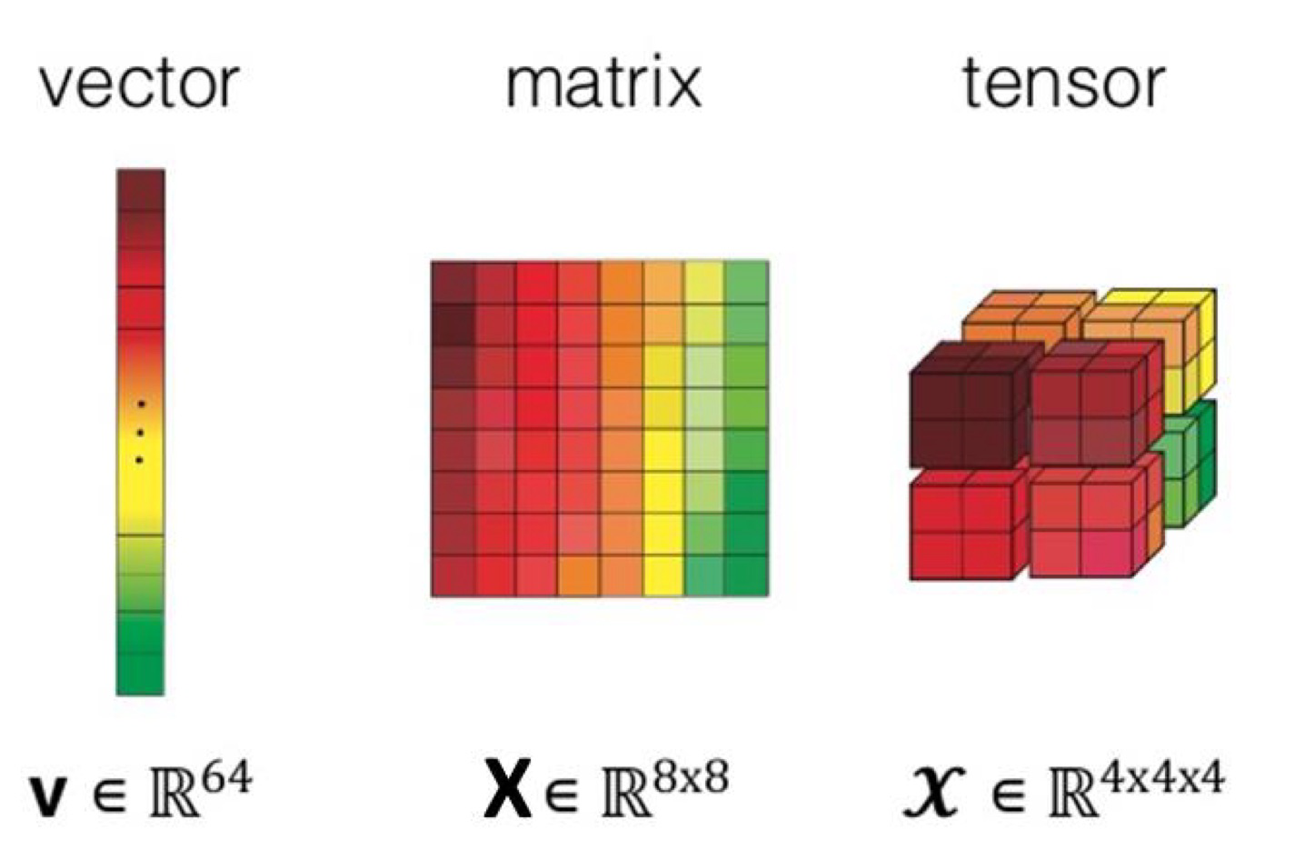
- Color images are typically stored as $n \times m \times 3$ tensors (arrays) - Red, Green, and Blue brightness values.
-
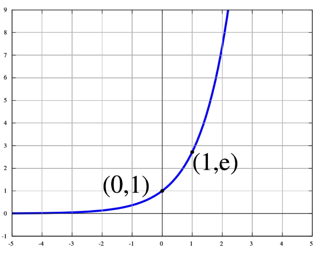
Exponential Function exp(x)
- $e^x = \exp(x)$
-
The exponential function $\exp(x)$ is defined as the power to which the number $e$ (approximately 2.71828, and known as Euler’s number) must be raised to yield $x$. Thus, $e^x = \exp(x)$.
-
Differentiability and Continuity:
- Continuous and differentiable across the entire real line.
- The derivative of $\exp(x)$ is $\exp(x)$ itself, which is a unique property and makes it extremely useful in differential equations and calculus.
- $K(x_i, x_j) = \exp\left(-\frac{|x_i - x_j|^2}{2\sigma^2}\right)$
- Continuous and differentiable across the entire real line.
- Multivariate Gaussian / Normal Distribution
- $m$ \indicates the mean of the $d$ -dimensional Gaussian}
- $\Sigma$ indicates the covariance matrix
- $f(\mathbf{x}) = \frac{1}{\sqrt{(2 \pi)^d \vert \Sigma \vert}} \exp\left(-\frac{1}{2} (\mathbf{x} - \mathbf{m})^T \Sigma^{-1} (\mathbf{x} - \mathbf{m})\right)$
- Vectorization for Making Code Fast
- Avoid for-loops if possible
- Try to directly implement algorithms using matrix and vector operations
- Parallelization is always important
2. Supervised Machine Learning
- After seeing a bunch of examples (Input space- $\mathbf x$, Output Space-y), pick a mapping $F:\mathbf x \rightarrow y$ that accurately replicates the input-output pattern of examples.
- With continous values $\rightarrow$ Regression
- Predicting class labels $\rightarrow$ classifier
- How well does the model $F$ work after training?
- Evaluate $F$ on the test data to get the generalized results
- Error for Regression (predicting continuous variables)
- Error measures to use when trying to predict real values instead of discrete values used in classification
- Mean Squared Error is the most common one
- $MSE = \frac{1}{N} \sum^N_{i=1} \Vert F(\mathbf X_i) - \mathbf y_i \Vert ^2 _2 $
- $MSE = \frac{1}{N} \sum^N_{i=1} \Vert F(\mathbf X_i) - \mathbf y_i \Vert ^2 _2 $
- Discrete Output Space
- With a discrete output space $\rightarrow$ classifiers
- class $\rightarrow $ labels or categories
- Nominal variables
- With a discrete output space $\rightarrow$ classifiers
- Classification Error and Accuracy (Predicting discrete variables )
- Accuracy = Total Correct / Total
- Error Rate = 1-accuracy
- For class imbalanced datasets, often deed to compute per-class accuracy statistics
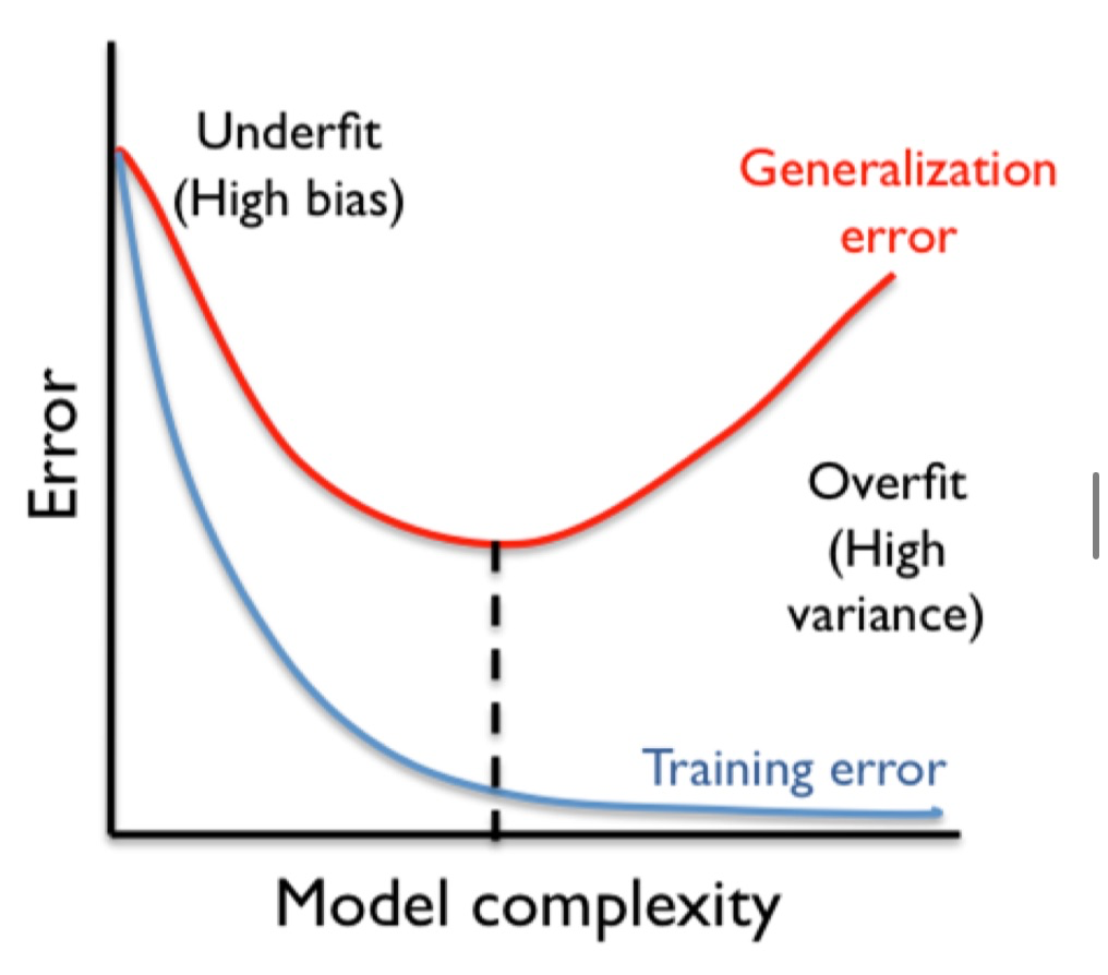
- Overfitting and Underfitting
- Overfit: if the training perforance is much greater than the testing performance
- Underfit: if the model isn’t powerful enough to derive the input-output relationship
- Regularization: mtethods for reducing overfitting
- Quantity of Data
- More labeled data, better model we can settle
- Data Augmentation
- Free way to get “more” data
- Random crops, rotations, flips, noise injection, color modifications and many others
3. Reveiw of Multi-Layer Perceptron
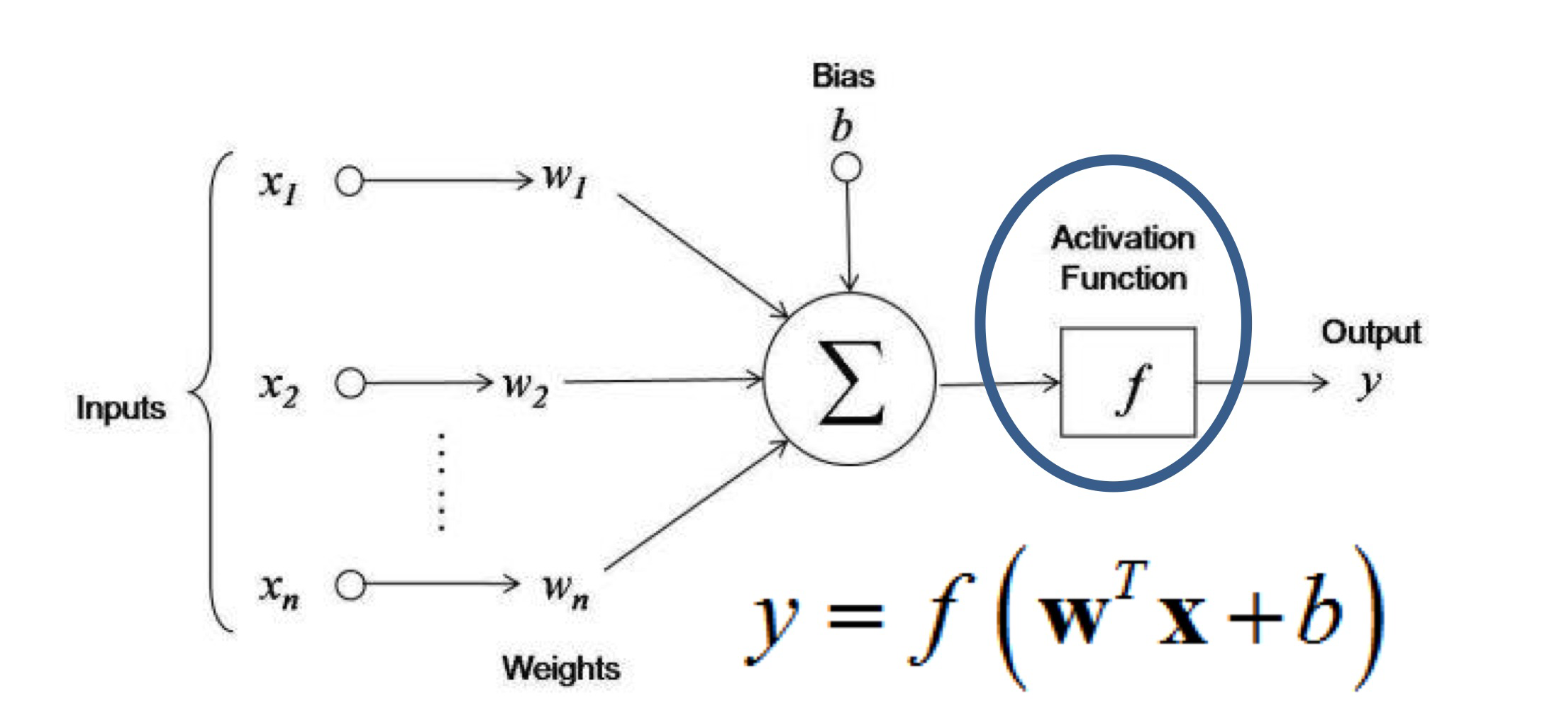
- The Artificial Neuron
- $y=f \big( \mathbf{w}^T \mathbf{x} + b \big)$
- Can use it for classification or regression tasks
- Activation function needs to be chosen for the task
- It constrains the output range
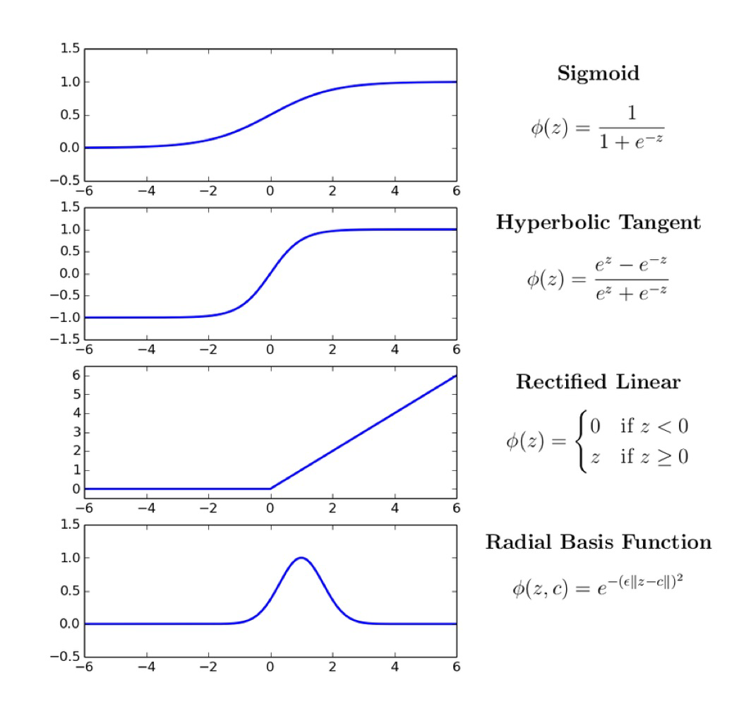
- Some common Activation Functions
-
Logistic Sigmoid Activation Function (most common)
- Forces output to be between 0 and 1
- Used for classification
-
Hyperbolic Tangent Activation Function (most common)
- Forces output to be between -1 and 1
-
Rectified Linear Activation Function
- Output between 0 and postiive infinity
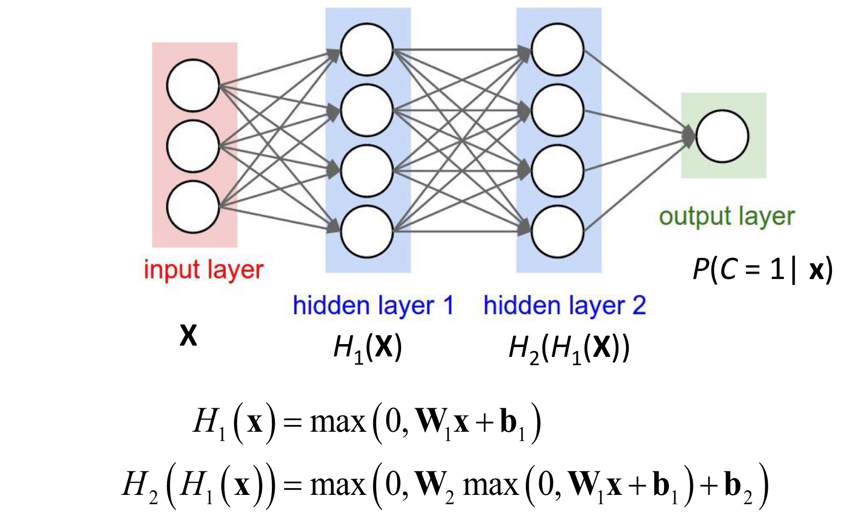
- MLP
- Each layer of units $\rightarrow$ matrix multiplication
- Unit’s weights $\rightarrow$ a row of a weight matrix
- Why Activation Functions?
- Without activation functions, will not get anny additional non-linearity in a MLP
- Two linear layers can just be combined into one.
- Without activation functions, will not get anny additional non-linearity in a MLP
- Model Capacity for Parametric Models
- Model capacity ( $\approx$ number of parameters)
- Greater model capacity $\approx$ more parameters in the model
- Bigger capacity $\rightarrow$ need more training data to train the model to avoid overfitting
- Low capacity $\rightarrow$ under-fit the training data significantly
- In a Neural Netrowors: More neurons = more capacity
- Linear classifier $\rightarrow$ low capacity
- Deep neural network $\rightarrow$ lot of capacity
- Model capacity ( $\approx$ number of parameters)
-
How to find Parameters $\mathbf w$ (weights) and $b$ (bias)
- Training : to identify good values for $\mathbf w$ and $b$
-
Fitting: for parametric models like neural networks
- Adjust the result with a loss function
- Loss Function (Cost Function, Error Function)
- Aim to minimize the loss function on the training data (lower training loss)
- Depends on what is the type of the model - regressions vs. classification
- Aim to minimize the loss function on the training data (lower training loss)
- Optimization Loss Landscape
- Find the global minima
- Weight Initialization
- Random initialization: All units all initialized from some random distribution
- Optimal distribution varies depending on activation function
- Poor initialization will impact trining greatly
- Transfer initialization: Take weights from another neural network trained on similar inputs from a large dataset.
- Random initialization: All units all initialized from some random distribution
- Bias Initialization
- Hidden layer bias is typcally initialized to Zero
- Output layer bais can be initialized from data for regression set it to the mean of the output vectors in training data $\rightarrow$ reduces “hockey Stick” loss curve
- Activation Functions & Loss Functions
- Activation functions define the outputs of the unit
- Output layer activation functions & loss functions : closely related
- Linear activation function for the out put is typically paired most often with:
- L2 Loss
- Huber Loss
- Logistic Sigmoid function for output is typically paired with:
- Binary cross-entropy loss (BCE Loss)
- Softmax for mutually exclusive classifcation
- Cross-entropy loss
- Linear activation function for the out put is typically paired most often with:
-
Gradient Descent
- First-order iterative optimization algorithm for finding a local minimum of a fucntion
- For finding the local maximum of a function $\rightarrow$ gradient ascent
- A procedure for minimizing a loss function to find the network’s parameters
- Compute partial derivates of the loss function with repsect to network parameters to give us the slope that telss us what direction to change each parameter get closer to the minima
- $w \leftarrow w - \eta \frac{\partial \text{Loss}}{\partial w}$
- $\eta$ is the learning rate
- Backpropagation: Gradient descent for Multi Layer Networks
- Use gradient descent to change the parameters $\mathbf w$ to reduce the loss
- Epochs & Loss Curves
- Gradient descent makes small changes to parameters to improve loss
- Many small changes are needed
- Epoch: An entire gradient descent pass through the whole training dataset
- Train loss should go down as a function of epochs
- Gradient descent makes small changes to parameters to improve loss
-
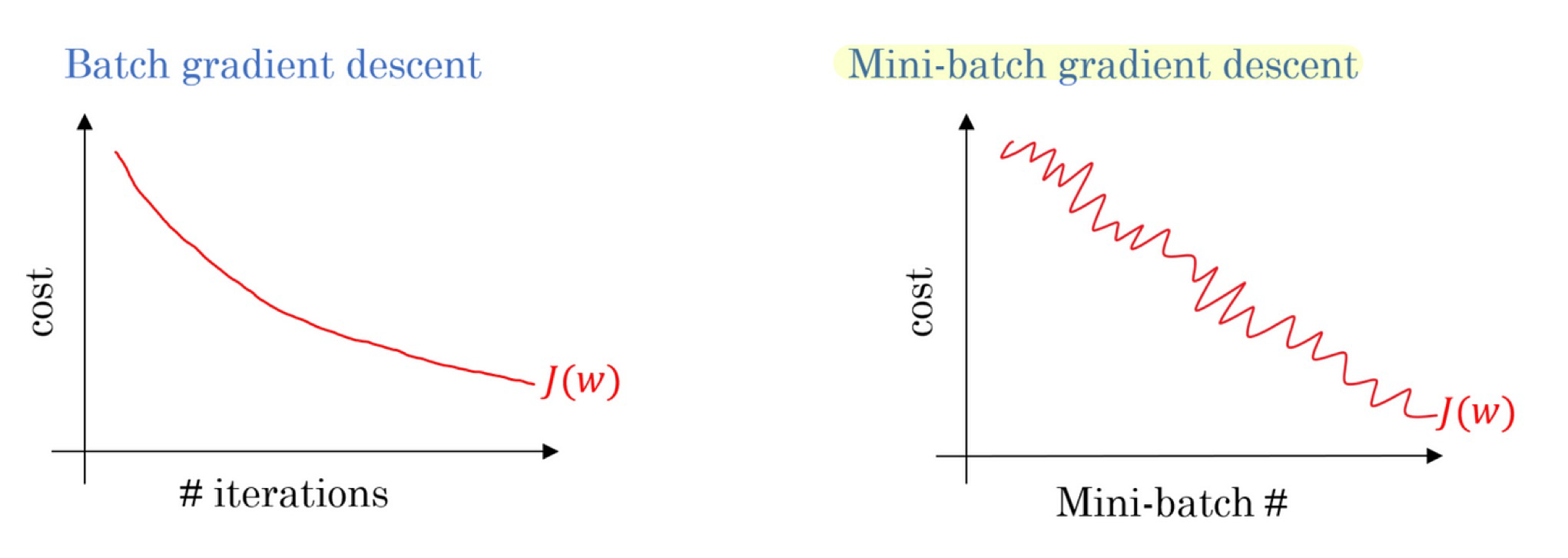
When should we update Parameters?
-
SGD: Compute update individually for each the N training instances (N updates in an epoch)
-
Full Gradient Descent: Update after seeing all the instances in the training set (1 update of in an epoch)
-
Mini Batch Gradient Descent: for deep learning
- Update N / M times, where M is the batch size
-
-
Adam
- Adapts the step sizes for different parameters
- Automatically adjusts the learning rate for each parameter based on the history of gradient
- Adam keeps track of two things:
- The average gradient (the “first moment”) – similar a running average of the direction
- The average of the squared gradients (the “second moment”) – how steep or flat the terrain is overall
- If the terrain is very steep in one direction (meaning large gradients), Adam will take smaller steps in that direction. if the terrain is flatter in another direction (smaller gradients), Adam will take larger steps.
- Relationship between Minibatch Size and Learning Rate
- When increasing the batch size, the optimal learning rate will change, and this depends on the optimization algorithm
- For SGD: When batch size increases by $k$, multiply the learning rate by $k$.
Leave a comment