
Day68 Deep Learning Lecture Review - Lecture 3
Neural Net Zoo: Transformers, Recurrent Neural Networks (RNNs) and Graph Neural Networks (GNNs)

We will review several high-level neural network architectures, which are all based on the MLP.
Fully-Connected Networks (MLPs) – Revisiting
- MLP is a class of fully connected feedforward neural networks. It consists of input layers, one or more hidden layers, and an output layer. Every node (neuron) in one layer is connected to every node in the next layer, hence the term “fully connected.”
- Critical Characteristics of MLP:
- General Purpose: MLPs apply to a range of tasks, including classification and regression. However, they do not naturally leverage data structures like images or time series.
- Fixed Input Size: MLPs require fixed-size input data (flattened into a vector), so they don’t naturally handle high-dimensional data like images without preprocessing.
- Lack of Spatial Awareness: MLPs do not consider the spatial structure of the data, making them less efficient for tasks like image recognition, where local relationships between pixels are essential.
- MLPs have been extended to handle other forms of data.
- It is often used in other networks.
- Sequential inputs and sets (text, audio, etc.): RNNs (many types), Transformers (many types)
- Graphs: Graph neural networks (many types)
- Images and Video: Convolutional Neural Network, Vision Transformers
- Every type of neural network architecture features layers with specific characteristics.
- You can combine them freely.
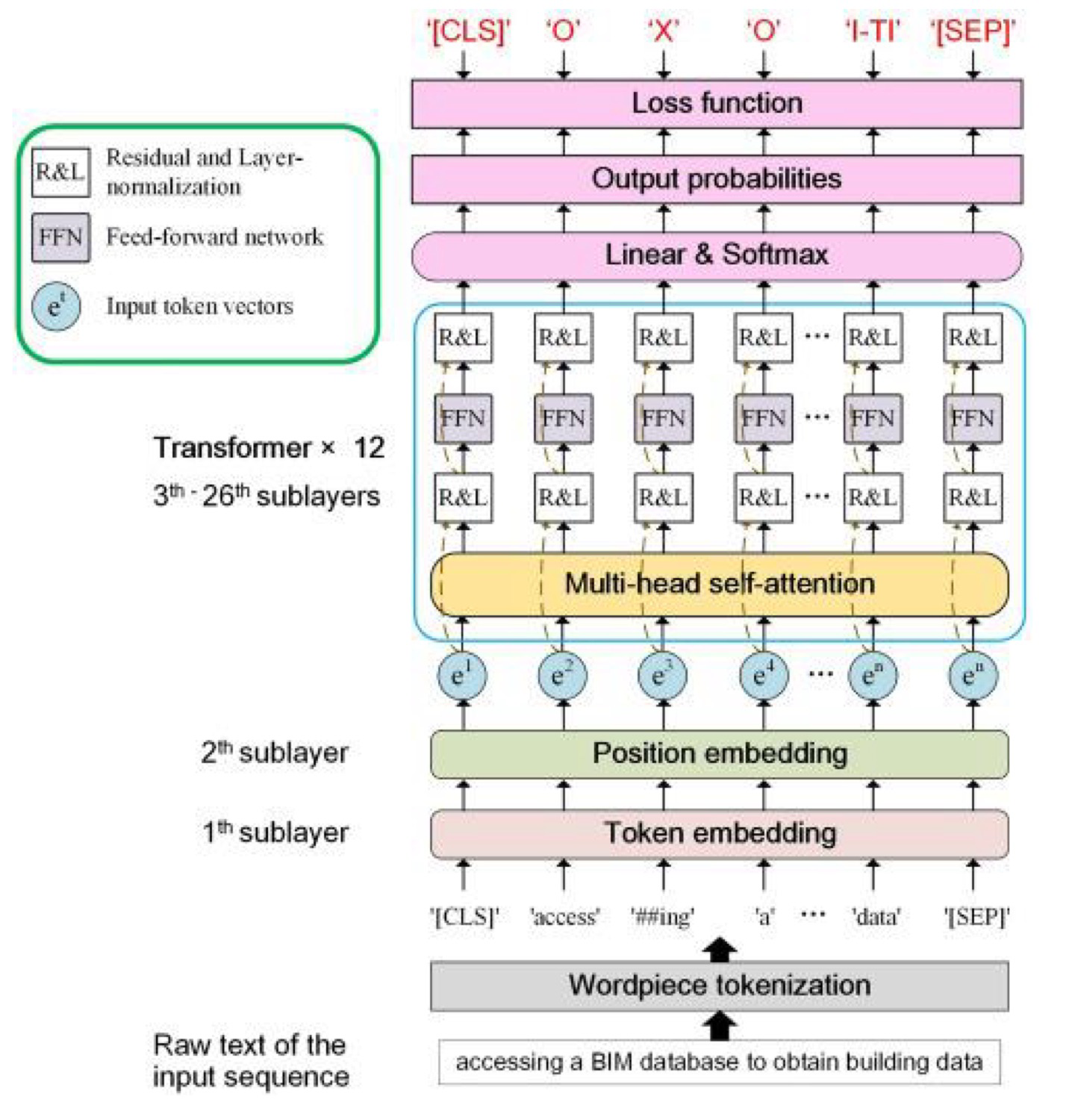
Transformers
- Transformers for Variable Length Sequences
- It can be used for sets of data and sequential data.
- Each input consists of N $d$-dimensional vectors, where $N$ is variable (sequence length).
- Uses weight sharing (same weights for each sequence element) and self-attention.
- Transformers Preserve Input Topology
- If we give a transformer layer $N$ vectors in a sequence, it will produce $N$ corresponding coutputs.
- The self-attention layer modulates the processing such that all other locations in the sequence modulate each location.
-
Transformer vs. Fully connected MLP Network
Features Fully Connected MLP Transformer Unit Input Vector $N$ $d$-dim Vectors Unit Output 1 number (scalar) $N$ $b$-dim Vectors Architecture Layers of densely connected neurons. Based on self-attention mechanisms. Encoder-decoder structure. Processing Processes all sequence parts simultaneously. Processes inputs independently; lacks sequence awareness. The $N$ inputs are often called “tokens”
Recurrent Neural Networks
- Recurrent Neural Networks (RNNs)
-
Used for sequential data, just like transformers
-
Hard to parallelized compared to transformers
-
Source: IBM-What is RNNs?
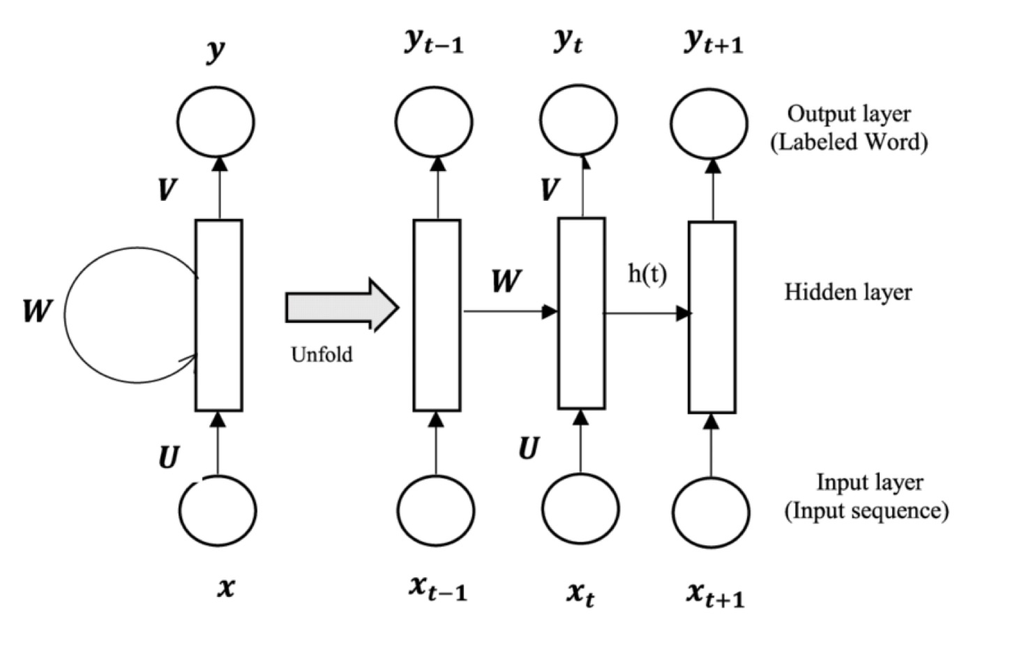
Recurrent Neural Networks (RNNs) are a class of neural networks specifically designed for handling sequential data.
- Unlike feedforward neural networks, which assume inputs are independent of each other, RNNs have connections that form cycles, allowing them to retain information from previous time steps.
Key Features of RNNs
- Sequential Data Processing: RNNs are designed to handle sequential or time-dependent data, such as time series, natural language, or video frames. They maintain a hidden state that captures information about previous time steps, enabling them to model dependencies over time.
- Hidden State: The key feature of RNNs is the hidden state, which acts as memory. The hidden state at each time step is updated based on the input at that step and the hidden state from the previous step, allowing the network to carry forward important information.
- Shared Weights: RNNs use the same weights across all time steps, which makes them more efficient when processing sequences of arbitrary length. This weight sharing allows them to generalize across different time steps in the sequence.
- Feedback Loops: RNNs have feedback loops that enable the network to incorporate information from previous time steps. This looping mechanism gives RNNs the ability to remember past inputs, making them suitable for tasks where context from earlier inputs is important.
How RNNs Work
RNNs process inputs sequentially, maintaining a hidden state that carries information from previous steps. At each time step, the network performs the following operations:
- Input: Receives an input vector (e.g., a word in a sentence).
- Hidden State Update: Updates the hidden state based on the current input and the previous hidden state.
- Output: Produces an output (e.g., predicting the next word in a sequence or classifying the sentiment of a sentence).
For long sequences, RNNs face challenges such as the vanishing gradient problem, which LSTMs and GRUs aim to address by adding mechanisms to retain and forget information selectively.
Comparison with Other Neural Networks
- RNN vs. CNN: While CNNs are good at processing data with grid-like structures (e.g., images), RNNs are better suited for sequential data (e.g., text or time series). CNNs are spatially focused, whereas RNNs are temporally focused.
- RNN vs. MLP: MLPs assume that the inputs are independent, which makes them unsuitable for sequential data. RNNs, on the other hand, explicitly model dependencies between inputs over time.
Limitations of RNNs
- Vanishing Gradient Problem: When training on long sequences, the gradients during backpropagation can shrink, making it hard for RNNs to learn long-term dependencies.
- Training Difficulty: RNNs are harder to train and often require specialized architectures like LSTMs or GRUs for better performance on long sequences.
Graph Neural Networks (GNNs)
Graph Neural Networks (GNNs) are a type of neural network designed specifically to work with graph-structured data.
In contrast to traditional neural networks like Convolutional Neural Networks (CNNs) or Recurrent Neural Networks (RNNs), which work with grid-like data structures (e.g., images or sequences), GNNs are designed to process and learn from data where relationships between entities can be represented as nodes and edges in a graph. This makes GNNs well-suited for tasks that involve understanding complex relationships, such as social networks, molecular structures, or knowledge graphs.
Key Concepts in GNNs
- Graph Structure:
- A graph consists of nodes (or vertices) and edges (connections between nodes). Nodes represent entities, and edges represent relationships between them. GNNs learn to propagate and aggregate information over this graph structure.
- Message Passing:
- GNNs operate based on a process called message passing. At each layer of the network, nodes update their representations by exchanging information (messages) with their neighboring nodes. The updated node representation is derived from both the node’s own features and the features of its neighbors.
- Message passing occurs iteratively across several layers, allowing information to propagate across the entire graph and enabling the model to capture both local and global dependencies.
- Node Embeddings:
- After multiple layers of message passing, each node in the graph has a learned representation or embedding. This embedding contains both the features of the node itself and information aggregated from its neighboring nodes, allowing the GNN to capture the graph structure and relationships.
- Graph-Level and Node-Level Tasks:
- GNNs can be used for a variety of tasks, including:
- Node classification: Predicting the labels of individual nodes (e.g., classifying users in a social network based on their connections).
- Link prediction: Predicting whether a connection (edge) exists or will exist between two nodes (e.g., recommending friendships in a social network).
- Graph classification: Assigning a label to an entire graph (e.g., determining the chemical properties of a molecule based on its atomic structure).
- GNNs can be used for a variety of tasks, including:
Transfer Learning
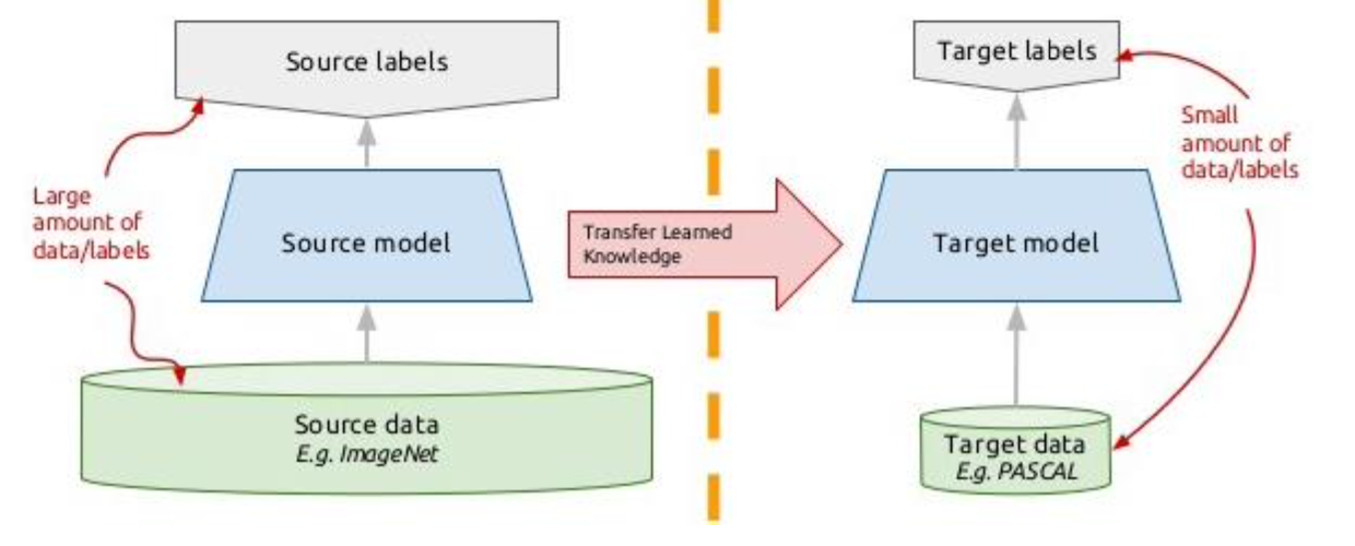
Transfer learning is a machine learning technique where a model developed for one task is reused as the starting point for a different but related task.
Instead of training a model from scratch, transfer learning allows leveraging pre-trained models that have already learned useful features, often speeding up training and improving performance, especially when labeled data is limited for the target task.
- Transfer learning typically starts with a model that has been pre-trained on a large dataset for a different task. For instance, models like ResNet, BERT, or GPT are pre-trained on massive datasets like ImageNet or large text corpora.
How Transfer Learning Works
- Base Task (Source Task):
- A model is trained on a large dataset for a base task. For example, a convolutional neural network (CNN) could be trained on the ImageNet dataset for image classification, learning features such as edges, textures, shapes, and object parts.
- Target Task:
- The pre-trained model is adapted for a different but related task, often with fewer labeled data. For example, a pre-trained CNN could be used to classify medical images by fine-tuning its weights on a much smaller dataset of medical images.
- Model Reuse:
- The knowledge learned in the base task is reused for the target task by either:
- Freezing some layers of the model and fine-tuning the rest, or
- Replacing the last layer(s) with a new one suited for the target task and fine-tuning the entire model.
- The knowledge learned in the base task is reused for the target task by either:
Types of Transfer Learning:
- Inductive Transfer Learning:
- In inductive transfer learning, the target task is different from the source task, but labeled data is available for the target task. The pre-trained model is fine-tuned on the labeled data for the new task. Example: Using a pre-trained ImageNet model to classify X-ray images.
- Transductive Transfer Learning:
- In transductive transfer learning, the target task is the same as the source task, but the domains (datasets) are different. Example: Using a pre-trained language model like BERT trained on Wikipedia to classify text in a specialized domain, such as legal or medical text.
- Unsupervised Transfer Learning:
- In unsupervised transfer learning, both the source and target tasks are unsupervised, meaning there are no labels. This type of transfer learning focuses on transferring feature representations across domains.
Leave a comment