Day72 Deep Learning Lecture Review - Lecture 4

📚 The Start of Recording TIL Summer ‘24 : Why Did I Start This Project? 🚀

🔔 Don't Miss: Continous Records of TIL '25 (Still On-Going!) 🌟

✨ A New Chapter in TIL '25: Reflecting, Growing, and Moving Forward 📖

Brief Explanation of Basic Algebra and Machine Learning

A very, very brief summary for the review of lectures three and four!

Linear Algebra

• Vector Norm: a function that takes a vector as input and outputs a single non-negative real number to show how significant that number is.

• Error for Regression: Error measures to use when predicting real values instead of discrete ones used in classification. MSE (Mean Squared Error) is the most common one.

• Error for Classification: Error and Accuracy (Predicting discrete variables)
  

Basic Machine Learning

• Underfitting: the classifier isn’t robust enough to model the input-output relationship.

• Overfitting: if the training performance is much more excellent than the testing performance
  • Regularization reduces overfitting.
• Data Augmentation: to get more data
  
  

Multi-Layer Perceptron (MLP) Networks: Weights, bias, and activation function

Common Activation Function:

• Linear activation function: just an identity function / used for regression

• Logistic sigmoid activation function: forces outputs to be between 0 and 1/ used for classification

• Hyperbolic Tangent Activation: Forces output to be between -1 and 1

• Rectified Linear Activation function: output between 0 and positive infinity.

• Without activation functions, you do not get additional non-linearity in an MLP.
  
  

Loss Function

• Need to measure how good a given w and b are
• We do this with a loss function.
• Measures how good a system is given its current parameter setting
• We want to minimize the loss function on the training data (training loss)
• As activation functions define the unit's outputs, the output layer activation function and loss functions are closely related.
• Linear activation function for the output is typically paired most often
  • L2 loss, Huber loss
• Logistic Sigmoid function for output is typically paired with
  • Binary Cross-Entropy loss (BCE loss)
• Softmax for mutually exclusive classification
  • Cross-Entropy loss
    
    
• Gradient descent is a procedure for minimizing a loss function to find the network’s parameters. n is the learning rate.

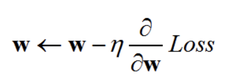
• Compute partial derivatives of the loss function concerning network parameters to give us the slope, which tells us in which direction to change each parameter to get closer to the minima.

• Backward Propagation: use gradient descent to change the parameters w to reduce the loss.

• SGD: taking small steps down a hill to find the lowest point.

  
  
  

• Gradient descent makes small changes to parameters to improve loss.
• An entire gradient descent passing through the training dataset is called an epoch.
  
  
  

When should we update the Parameters?

• SGD: Compute update individually for each of the N training instances.
  • N updates in an epoch.
• Full Gradient Descent: Update after seeing all the instances in the training set.
  • 1 update of in an epoch
• We use (mini) batched gradient descent for deep learning.
  • Update N / M times, where M is the batch size and M is the batch size.
    
    

Adam

• A more sophisticated version of SGD that adapts the step sizes for different parameters
• Adam automatically adjusts the learning rate for each parameter based on the history of gradients. This speeds up training.
• Adam keeps two things:
  • The average gradient
  • The average of the squared gradients
    
    

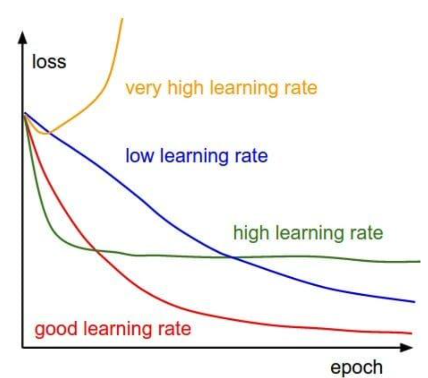
Minibatch size and learning rate

When we increase the batch size, our optimal learning rate will change, depending on the optimization algorithm.

• For SGD: When batch size increases by k, multiply the learning rate by k.
  
  

Checkpoint Selection

• Often, we choose the model with the best validation performance (e.g., lowest validation loss)

Need to know

• Evaluation: Accuracy, Error, AUC, Confusion Matrix, Decision Boundaries, etc.
• MLPs: Loss functions, activation functions
• Activation functions: Logistic Sigmoid, ReLU, Linear
• Loss functions: L2, Cross-entropy
• Regularization: Weight decay, early stopping/checkpoint selection, dropout
• Backpropagation: Gradients, Epochs, Batches
  
  
  

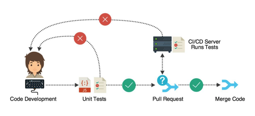
MLops Using tests

• CI/CD Pipelines are used.
  • Code is built
  • Tests execute after building (CI)
  • Tests fail, there is a problem.
  • Deploy (CD)

• Containers
  • Docker / Kubernetes
    • Docker containers are built from the images, which is where your code lives
    • Docker Images are the “source code” for creating a container

Tests for ML Systems

• Pre-train Tests: Tests that do not need the system to be trained.
  • Check the shape of your model output and ensure it aligns with the labels in your dataset
  • test with a very small dataset and make sure you can overfit it
  • Steps
    • Make sure the optimizer can reduce the loss to near zero.
    • If it cannot something is wrong, probably with the optimizer.
• Post-train Tests: Tests that need the system to be trained.
  • Invariance test: check for consistency in the outputs despite reasonable perturbations
  • Robustness test: measure the robustness of outputs
  • Directional Expectation tests
  • Minimum functionality tests
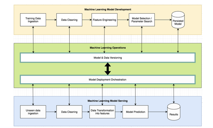
• Version everything: Datasets, Experiments, Models
  
  

Workflow Orchestration

• Automating machine learning workflows.
• What is workflow orchestration?
• -> Changing pre-processing, training, and evaluation systems together

Side Note: Sequential & Non-Sequential Data

When working with sequential data (such as time series, speech, and natural language), machine learning (ML) and deep learning (DL) models that account for temporal or sequential relationships are used. For non-sequential data (like images, tabular data, or static observations), models that treat each input independently are employed.

• Sequential Data Models

  1. Recurrent Neural Networks (RNNs): RNNs are explicitly designed for sequential data. Their connections loop back, allowing them to retain information from previous inputs, making them suitable for data where context or memory is essential.

     • Commonly used: Time-series forecasting, Natural Language Processing, Speech recognition
     • Limitations: Vanishing gradients
       
       

  2. Long-Short-Term Memory (LSTM): LSTM is a variant of RNNs that includes a memory cell and gating mechanisms (input, forget, and output gates), allowing the network to remember longer sequences of information. This solves the vanishing gradient problem that standard RNNs face.

     • Commonly used: Text generation, machine translation, and speech synthesis
       
       

  3. Gated Recurrent Units (GRUs): GRUs are a simplified version of LSTMs. They use fewer gates but still retain the ability to remember long sequences. They are computationally more efficient and often perform similarly to LSTMs.

     • Commonly used: Similar to LSTMs, including sentiment analysis, machine translation, and sequence classification.
       
       

  4. Transformers: Transformers are a more recent development that uses self-attention mechanisms to process sequential data rather than relying on recurrent connections like RNNs. They can handle longer sequences much more efficiently because they don’t process data step-by-step but in parallel. Transformers also excel in learning context over long sequences.

     • Commonly used: Text translation(e.g., GERT, GPT), summarization, and question answering
       
       

• Non-Sequential Data Models

  1. Feedforward Neural Networks (FFNNs): FFNNs process input data without considering any sequence. They pass data from input to output without memory or recurrence, making them ideal for independent, non-temporal data.

     • Commonly used: Classification of tabular data, regression tasks, and simple pattern recognition

  2. Convolutional Neural Networks (CNNs): CNNs are primarily used for spatial data (such as images), where nearby pixels are related. CNNs use convolutional layers to capture spatial hierarchies and are excellent at identifying local patterns (like edges or textures).

     • Commonly used: Image classification, object detection, medical image analysis.

     
     
     

• Machine Learning Techniques for non-sequential models

  1. Random Forests (RF): Random Forest is a traditional machine learning algorithm that operates by creating multiple decision trees and combining their results. It treats each data point as independent and is not designed for sequential relationships.
     • Commonly used: Classification and regression on tabular data, such as customer churn prediction or medical diagnoses.
  2. Support Vector Machines (SVMs): SVMs are designed to find the optimal hyperplane that separates different classes in high-dimensional space. They treat each input independently and don’t consider any temporal or sequential order.
     • Commonly used: Text classification, image classification, and small-to-medium-sized tabular datasets.
  3. XGBoost: XGBoost is a gradient-boosting algorithm that builds models sequentially but treats each data point independently. It is highly effective for non-sequential data.
     • Commonly used: Tabular data prediction tasks like fraud detection, ranking problems, or sales forecasting.