Day73 Deep Learning Lecture Review - Lecture 5

📚 The Start of Recording TIL Summer ‘24 : Why Did I Start This Project? 🚀

🔔 Don't Miss: Continous Records of TIL '25 (Still On-Going!) 🌟

✨ A New Chapter in TIL '25: Reflecting, Growing, and Moving Forward 📖

Transformers and Foundation Models: GELU, Layer Norm, Key Concepts & Workflow

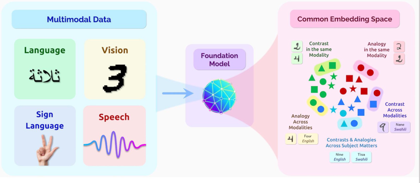
Foundation models are large-scale, pre-trained models used as the basis for a wide range of tasks in machine learning, especially in Natural Language Processing (NLP), Computer Vision (CV), and other areas. They are trained on diverse, extensive datasets using unsupervised or self-supervised learning techniques. These models can be fine-tuned for specific tasks using smaller datasets. They are huge, often containing billions of parameters, and can be applied to many different functions without being re-trained completely.

Foundation models are pre-trained in a self-supervised manner, which means they learn representations without requiring labeled data. Following pre-training, they can be fine-tuned on a smaller, task-specific dataset. They mark a shift toward building generalized AI systems that can solve diverse problems without task-specific retraining. However, their development and deployment come with challenges, such as resource-intensive training, ethical considerations, and biases inherent in the training data.

GELU Activation Function

The GELU (Gaussian Error Linear Unit) activation function is a smooth, non-linear function primarily used in neural networks. It is often used in models like BERT (Bidirectional Encoder Representations from Transformers) and other transformer-based architectures because it performs superiorly to traditional activation functions such as ReLU (Rectified Linear Unit).

• It is used in most transformer models and now in many CNN and MLP architectures.
• Doesn’t have a dying ReLU problem. Smoother Activation near zero, Probabilistic Behavior, Differentiable in all ranges, and allows (small) gradient in the negative range.
  • Unlike ReLU, which is piecewise linear and has discontinuities, GELU is a smooth and differentiable function, which is beneficial for optimization in deep learning models.
  • GELU’s smoother behavior allows gradients to flow more easily during backpropagation, especially for values near zero.
  • This reduces the chances of the model facing “dead neurons” that can happen in ReLU (where negative values are zeroed out entirely).
    

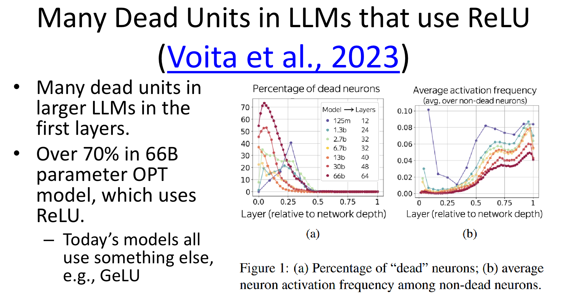
Image from: Kanan, C., "End-to-End Deep Learning," CSC477.01.FALL2024ASE Lecture Slides, University of Rochester, 2024.

Normalization Functions

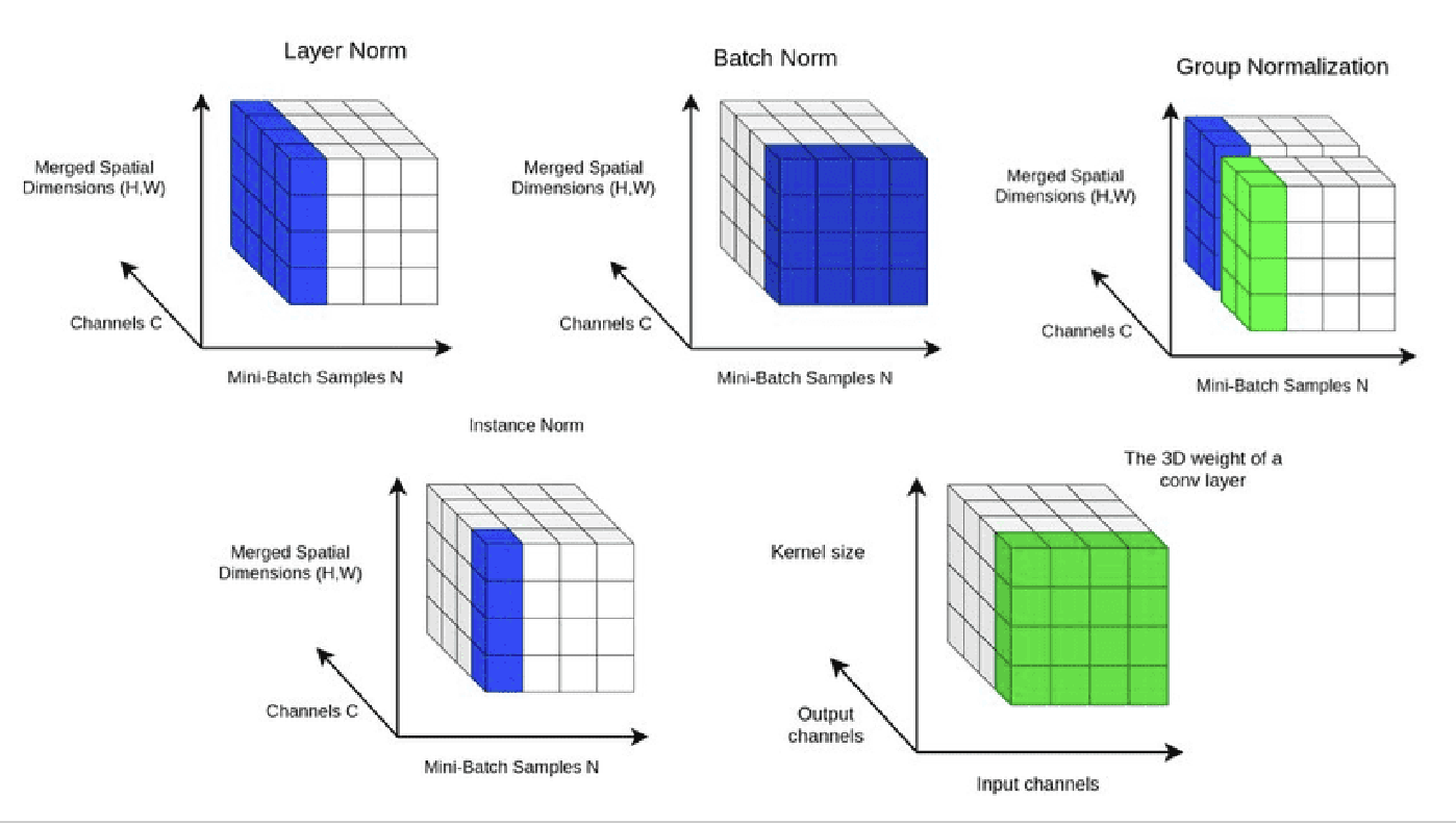
• Layer Norm
  • It normalizes across all features in a given layer. It applies normalization across the channels (C) and merged spatial dimensions (H, W) for each individual sample in the mini-batch.
  • It works well for non-sequential data and has applications in transformer architectures, where mini-batch normalization could be more effective.
• Batch Normalization
  • Normalizes over the mini-batch samples (N) and the spatial dimensions (H, W), but each channel (C) is normalized independently.
  • This normalization is applied per channel for a mini-batch. It is commonly used in CNNs to reduce internal covariate shifts, speed up training, and allow for higher learning rates.
• Group Normalization
  • Splits channels into groups and normalizes across each group and spatial dimensions.
• Instance Normalization: Normalizes for each sample and channel separately.
• Convolutional Weight: Shows how convolution kernels work across input and output channels.

• Layer Norm vs. Batch Norm
  • Layer Norm: Subtract mean of each input vector and divide by the vector’s standard deviation
  • Batch Norm: Subtract channel mean computed using all samples in batch, and then divide by channel standard deviation calculated using all samples in batch.
  • Layer norm is invariant to batch size.
  • Layer norm tends to make training slower.

Batch Norm is a Frequent Problem.

• Batch normalization (Batch Norm) has been a widespread technique in deep learning, primarily used to speed up training and stabilize neural network models. However, it also comes with some limitations and challenges.

  1. Dependency on Batch Size: Batch Norm’s performance highly depends on the batch size used during training. If the batch size is too small, the statistical estimates of the mean and variance may be inaccurate, leading to noisy gradients. It calculates the mean and variance of features across the mini-batch, and smaller batch sizes mean less accurate estimates of these statistics, potentially hurting model performance.

  2. Training vs. Inference Discrepancy: During training, batch normalization uses the statistics of the current mini-batch, but during inference (or testing), it uses running estimates (moving averages) of the batch statistics. These estimates might not perfectly match the actual statistics at inference time. The difference between training and inference statistics can lead to a performance drop at inference time, mainly when the model is sensitive to the exact distribution of features.

  3. Not Effective for Small Batches or Online Learning: Batch normalization struggles in settings where small batch sizes are required (e.g., huge models, memory-constrained environments) or in online learning (streaming data) scenarios. When using small batch sizes, the statistics are often noisy and unstable, which reduces the effectiveness of normalization. In online learning, applying the Batch Norm becomes impractical since the data comes in a stream and mini-batch statistics are unavailable.

  4. Batch Norm Doesn’t Work Well with Recurrent Neural Networks (RNNs): Batch normalization is less effective in Recurrent Neural Networks (RNNs) and other sequential models. In RNNs, the internal state is passed over many time-steps, and normalizing these sequences using batch statistics can interfere with the temporal dependencies in the data. Other normalization techniques, such as Layer Normalization, are typically preferred in RNNs and transformers because they work better in sequential models.

Side Note: Layer Norm

Layer Normalization (LayerNorm) is a normalization technique used in neural networks, particularly effective for models where the input is sequential, such as Recurrent Neural Networks (RNNs) and Transformers. Unlike Batch Normalization (BatchNorm), which normalizes across the batch dimension, LayerNorm normalizes across the features within each layer for each input, making it independent of the batch size.

For each input instance (or sample), LayerNorm normalizes the activations across all features (neurons) in a layer by calculating the mean and variance for the entire layer’s output rather than across a mini-batch. This ensures that the activations have a consistent distribution for each input, which helps stabilize and speed up the training process.

Transformers

The Transformer is a deep learning model architecture introduced in the “Attention is All You Need” paper by Vaswani et al. in 2017. It revolutionized the field of Natural Language Processing (NLP) and is now the backbone of many state-of-the-art models, including BERT, GPT, and T5. The Transformer is unique because it is based entirely on attention mechanisms, without relying on the recurrence (as in Recurrent Neural Networks, RNNs) or convolutions (as in Convolutional Neural Networks, CNNs). This allows it to handle longer-range dependencies and parallelize training more efficiently.

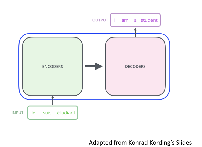
The conventional seq2seq model was composed of an encoder-decoder structure. Here, the encoder compresses the input sequence into a single vector representation, and the decoder generates the output sequence based on this vector representation. However, this structure has the downside of losing some information from the input sequence while compressing it into a single vector, and attention mechanisms are used to address this. But what if we create an encoder and decoder using only attention rather than employing it as a correction for RNN?

Critical Components of the Transformer:

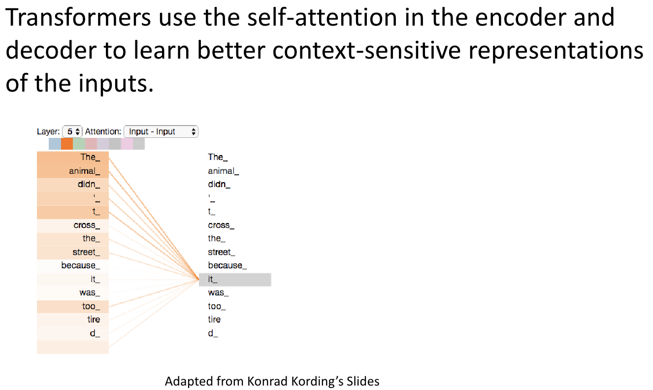
1. Self-Attention Mechanism

   • The Transformer’s most critical innovation is its self-attention mechanism. It enables the model to simultaneously attend to all words in a sequence rather than processing them sequentially, as in RNNs.
   • Self-attention computes a weighted representation of the entire input sequence, where the importance of each word in the sequence is calculated relative to all other words. This helps the model understand each word’s context by considering its relationships with every other word in the sequence.
     
     

2. Positional Encoding

   • Unlike RNNs, which have an inherent sense of order due to their sequential nature, the Transformer processes input in parallel. The model needs a natural understanding of word order or positional information.
   • The Transformer adds positional encodings to the input embeddings to encode this positional information, allowing the model to capture the order of words in the sequence.
     
     

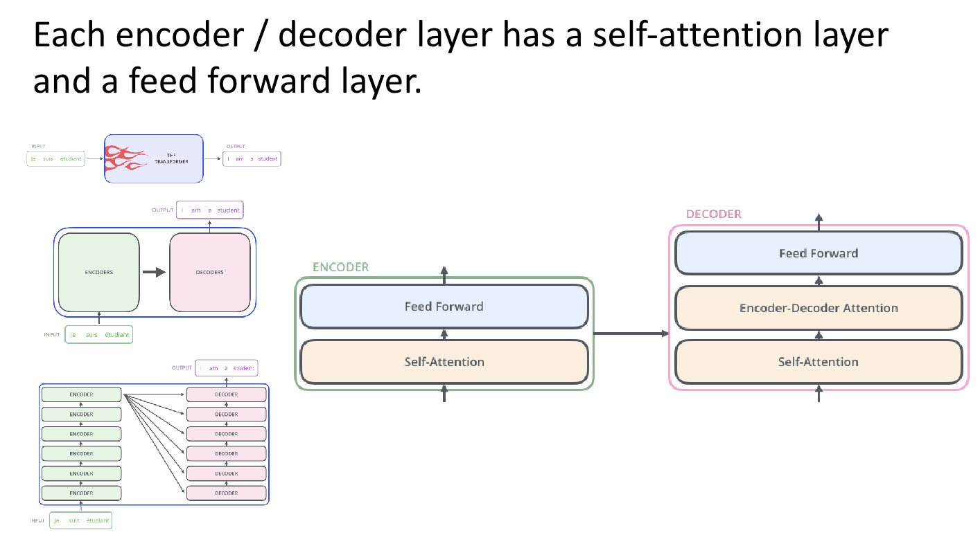
3. Encoder-Decoder Architecture

   • The original Transformer architecture consists of two main components.
     • Encoder: A stack of identical layers where each layer applies self-attention followed by a feed-forward network. The encoder’s job is to take in the input sequence and learn rich representations.
     • Decoder: Also a stack of identical layers, but in addition to self-attention, it uses cross-attention to attend to the encoder’s output.
       
       

   ​
   
   
   ​ </center>

4. Multi-Head Attention:

   • The Transformer uses multi-head attention, a mechanism applying several parallel self-attention operations. Each attention “head” focuses on different parts of the input sequence. The results are then concatenated and projected to get the final output.
   • This allows the model to learn different relationships between words (e.g., syntactic and semantic relations) from multiple perspectives.
     
     

5. Feed-Forward Network (FFN)

   • After applying self-attention, each encoder and decoder block has a feed-forward network, which is applied to each position independently. The FFN typically consists of two linear layers with a ReLU activation in between, allowing for non-linear transformations of the attention outputs.
     
     

6. Layer Normalization and Residual Connections

   • Each sub-layer (like self-attention and feed-forward networks) in the Transformer is followed by layer normalization and a residual connection. This helps with training stability and allows better gradient flow, which speeds up convergence.

Workflow of the Transformer

The Transformer consists of two algorithms- an encoder and a decoder.

The Transformer does not use RNNs but retains the encoder-decoder structure that, like traditional seq2seq models, receives an input sequence in the encoder and outputs an output sequence in the decoder. In the previous seq2seq structure, each encoder and decoder consisted of a single RNN with $t$-time steps; however, the encoder and decoder units comprise N components in the transformer. The paper proposes the Transformer used a total of 6 for both the encoder and decoder.

Explanation from: Wiki Docs in Korean

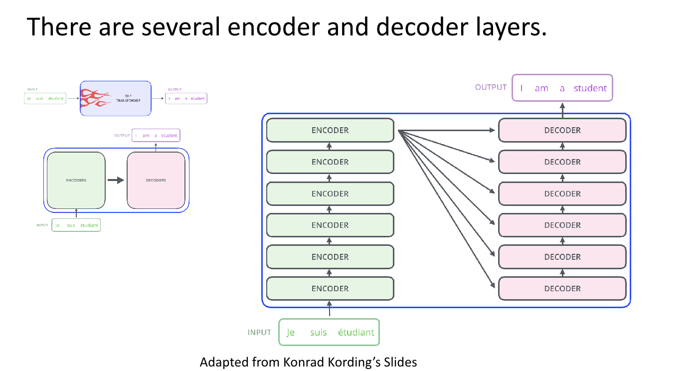
The image below shows the transformer structure where the decoder generates output results based on information received from the encoder. The decoder operates similarly to the traditional seq2seq structure, taking the start symbol <SOS> as input and continuing its computations until the end symbol is produced <EOS>. This demonstrates that although RNNs are not used, the encoder-decoder structure is still maintained.

Let’s start by gradually exploring the internal structure of the transformer. We’ll first comprehend the transformer’s input before diving into the encoder and decoder structure. The encoder and decoder of the transformer do not simply receive the embedding vectors of each word. Instead, they take adjusted values from the embedding vectors, which we will explore by expanding on the input section.

1. Input Embedding and Positional Encoding

   Before understanding the internals of a transformer, let’s first take a look at the inputs of a transformer.

   • RNNs were helpful in natural language processing due to the characteristic of RNNs that allows them to process input words based on their positions sequentially, enabling them to retain positional information.

   • However, since transformers do not receive word inputs sequentially, it is necessary to communicate positional information differently. To obtain positional information, transformers add positional encodings to the embedding vectors of each word and use them as input to the model, referred to as positional encoding.

   • Each word in the input sequence is converted into an embedding (vector representation). Positional encodings are added to these embeddings to provide information about the position of each word in the sequence.
     
     

2. Encoder

   • The input embeddings pass through the stack of encoder layers, which apply self-attention and feed-forward networks to transform the input into contextualized representations.

3. Decoder

   • In tasks like machine translation, the decoder receives the target sequence (e.g., the translation so far). It uses self-attention and cross-attention (To attend to the encoder’s output) to generate the next word in the output sequence.
     
     
   

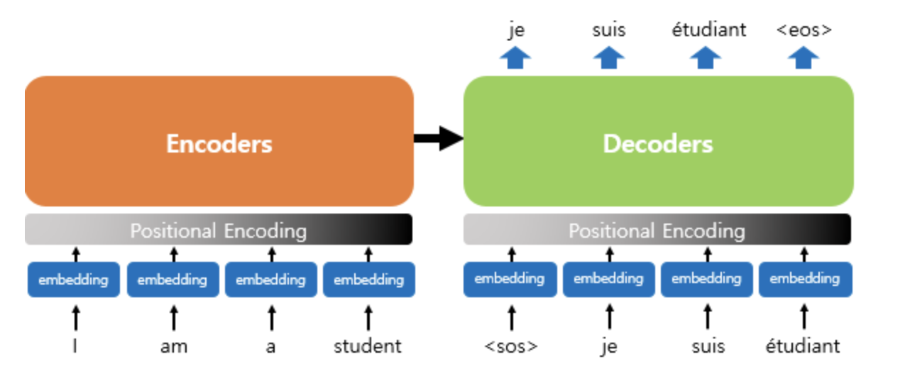
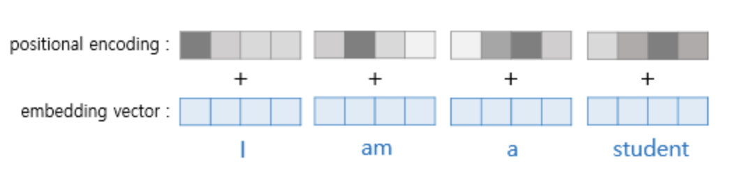
   As shown in the illustrations above, the positional encoding values are added to the embedding vectors before they are used as input to the transformer. The transformer employs two functions to assign the positional encoding values to the vectors.

   $PE_{(pos, 2i)} = sin(pos/10000^{2i/d_{model}})$
   
   $PE_{(pos, 2i+1)} = cos(pos/10000^{2i/d_{model}})$
   
   
   

   The transformer adds the values of the sine and cosine functions to the embedding vectors, thereby incorporating the words’ order information. Additionally, it is important to understand that the addition of the embedding vectors and positional encodings is performed through the addition operation between the sentence matrix created by the embedding vectors and the positional encoding matrix.

   

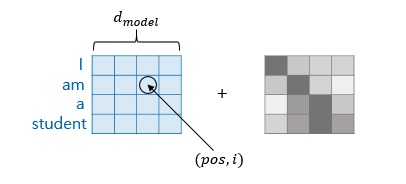
   The $pos$ indicates the position of the embedding vector in the input sentence, while $i$ signifies the index of the dimension within the embedding vector.

   According to the formula above, if the index of each dimension within the embedding vector is even, the sine function value is used; if it is odd, the cosine function value is used. Note that when $(pos, 2i)$ is involved, the sine function is utilized, while for $(pos, 2i+1)$, the cosine function is applied.

   Additionally, in the formula above, $d_{model}$ refers to the output dimension of all layers in the transformer, which is a hyperparameter of the transformer. The embedding vector also has the dimension of $d_{model}$; in the above diagram.

   Using the positional encoding method as described, the order information is preserved. For example, when the positional encoding values are added to each embedding vector, even if they are the same word, the values of the embedding vectors entering the transformer as inputs will differ based on their position in the sentence. Consequently, the input to the transformer will consist of embedding vectors that consider order information.
   
   

   We will further explore its structure in the next post.

4. Output

   • The decoder’s final output passes through a linear layer followed by a softmax to produce the probability distribution over the target vocabulary for the next word in the sequence.