Day88 Deep Learning Lecture Review - Lecture 10-12

📚 The Start of Recording TIL Summer ‘24 : Why Did I Start This Project? 🚀

🔔 Don't Miss: Continous Records of TIL '25 (Still On-Going!) 🌟

✨ A New Chapter in TIL '25: Reflecting, Growing, and Moving Forward 📖

Deep Learning & Numerical Precision(Floating Point), Hardware Considerations, and Distributed Model Training

Bus Bottleneck

A bus bottleneck refers to a situation in computer systems where the data bus, which connects different components (such as the CPU, memory, and peripherals), becomes a limiting factor for system performance. A bus is responsible for transmitting data between components, and when it cannot handle the volume of data being transferred, it becomes a bottleneck.

• Common Causes of Bus Bottlenecks
  • Limited Bandwidth: The data bus has a finite bandwidth, which defines how much data it can transfer per unit of time. Suppose the transmitted data exceeds the bus’s capacity, resulting in a bottleneck.
  • High Traffic Load: When multiple devices or components try to use the same bus simultaneously, the bus can become overwhelmed, leading to delays and slower data transmission.
• Solutions to Address Bus Bottlenecks:
  • Increasing Bus Bandwidth: Upgrading to buses with higher bandwidth can reduce bottlenecks. For example, PCIe (Peripheral Component Interconnect Express) can drastically improve component data transfer rates compared to older bus technologies like PCI or AGP.
  • Bus Architecture Optimization: Modern systems often use multiple buses (e.g., separate buses for CPU-memory communication and I/O devices) to reduce traffic on a single bus and avoid bottlenecks.
  • Parallel Bus Systems: Increasing the number of parallel data lines can improve throughput, as more data can be transmitted simultaneously.
• SXM (Scalable Matrix Extension) and NVLink can be used.
  
  

Floating Point

A floating point is a way to represent real numbers in a computer system using a finite number of bits.

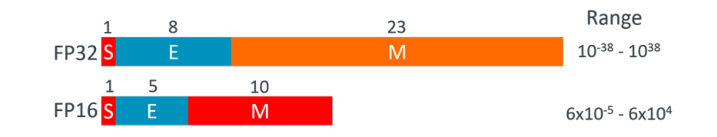
• FP32 is the 32-bit floating-point format commonly used in computer systems for numerical computations, following the IEEE 754 standard. FP32 (also known as single-precision floating point) uses 32 bits to represent real numbers, split into three components:
  • 1 bit for the sign: Indicates whether the number is positive (0) or negative (1).
  • 8 bits for the exponent: This encodes the scale of the number by representing the power of 2 multiplied by the number.
  • 23 bits for the mantissa (or significand): This represents the actual precision of the number.
    

• Half Precision: FP16

  • FP16 uses only 16 bits rather than 32 bits.
  • It has less precision and a smaller range of values.
  • FP16 is about twice as fast as FP32.
  • Weights in FP16 require half as much VRAM.
  • If we can train in lower precision (fewer bits), we would have more GPU memory available, and arithmetic operations would be faster as FP16 uses half the amount of RAM as FP32.
  • We could also use a bigger model and batch size, yielding a more significant speedup.

• Remember that we must also have a VRAM dedicated to 2x your model size.

  • – 1x is your model
  • – 1x is your optimizer: Momentum, Adam, AdamW, etc.
    
    
• Mixed Precision Training
  • We often encounter numerical problems when using FP16 everywhere. Although it is okay for the forward pass, it is insufficient for computing weight updates.
  • Mixed precision training combines FP32 and FP16 (or BFLOAT16 or TFLOAT32).
  • It enables shorter training times and lowers the memory requirements of training with bigger models, batch sizes, and inputs.
    
    
• Automatic Mixed Precision (AMP)
  • Using mixed precision arithmetic could enhance computational efficiency. Instead of relying solely on 32-bit floating point (FP32) operations, AMP dynamically scales between 16-bit floating point (FP16) and FP32 arithmetic during training.
  • Using FP16 for less critical calculations, AMP can reduce memory and speed up computations, especially on modern hardware like NVIDIA GPUs with Tensor Cores optimized for FP16.
    
    
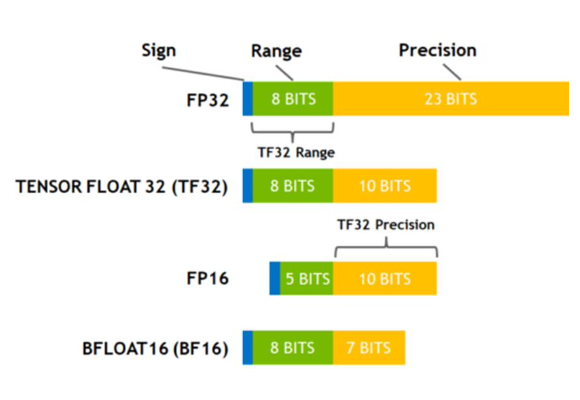
• BFLOAT16
  • bfloat16 (Brain Floating Point 16) is a 16-bit floating-point representation used primarily to accelerate deep learning tasks. Google introduced it, and hardware manufacturers like Intel and NVIDIA adopted it.
  • Unlike the standard 16-bit floating-point format (FP16), bfloat16 retains the same range as a 32-bit floating-point (FP32) format but with reduced precision. This makes it particularly useful in machine learning tasks, where having a wide dynamic range is essential, but accuracy can be sacrificed for faster computations.
    
    
• Tensor Float 32
  • TF32 offers a middle ground between FP32 and FP16 formats by balancing performance with precision.
  • It only offers 18 bits (NOT 32 bits) and the same dynamic range as FP32 and BFLOAT16, with the same precision as FP16, whereas BFLOAT16 has less precision than FP16.
    
    

• INT8

  • It refers to an 8-bit integer format used in machine learning and deep learning to represent numerical data.
  • INT8 quantization converts the weights and activations of a neural network from higher-precision formats (like FP32) into 8-bit integers.
  • Two essential methods are used:
    • Post-training quantization: Quantizing a model after it has been trained with floating-point values.
    • Quantization-aware training: Training the model while simulating quantized arithmetic, leading to better accuracy after quantization
  • Accuracy Loss: Since INT8 quantization reduces the precision of model weights and activations, it can slightly deteriorate model performance. This is particularly noticeable in models that rely on very fine-grained numerical precision.
    
    

Hardware Considerations

• Different GPUs support different precisions. Not all GPUs support bfloat16 or TF32. Some GPUs support special operations to enable faster mixed-precision training.

• Tensor Cores

  • Tensor cores can accelerate mixed precision training, but not all GPUs have them.
  • Accelerated cores for multiplying two FP16/BFLOAT16/TF32 matrices and adding an FP32/FP16/BFLOAT16/TF32 matrix, but the returned value can be in FP32.
  • Using Tensor cores for speed up can greatly reduce the GPU utilization by having BatchNorm in the code.
    
    

Prefetching

Prefetching is a technique used in computer systems to improve performance by *loading data into the cache or memory before the CPU or other components need it.

• Prefetching data loaders have the data loaded and transformed in a separate thread so that the GPU does not need to wait. This is what PyTorch’s data loader does.
• Dataloaders often allow for parallel data loading through multiple worker threads. This speeds up data retrieval, ensuring the model does not wait for data to be loaded during training and thus increasing training efficiency.
  • In PyTorch, setting num_workers=4 allows for parallel data loading with four worker processes.
• NVIDIA’s Data Loading Library (DALI) pipeline loads data on the CPU and then decodes it to the GPU, where it is augmented.
  • DALI supports data prefetching transparently with a queue to get batches ready ahead of time.
• FFCV
  • FFCV is a fast and efficient computer vision data-loading framework designed to optimize loading large datasets, especially for deep learning tasks. It aims to reduce bottlenecks caused by slow data loading, which often limits the performance of models on GPUs. FFCV speeds training and inference using efficient data storage formats and parallel data loading strategies.
  • In PyTorch, for example, FFCV can be an alternative to traditional data loaders like torch.utils.data.DataLoader. By converting datasets into FFCV’s format and using FFCV’s efficient data loader, training times can be significantly reduced, mainly when dealing with image datasets like ImageNet.
    
    
    

Activation (Gradient) Checkpointing

Activation (Gradient) Checkpointing is a memory optimization technique used in deep learning to reduce the memory footprint during model training, particularly for intense neural networks or models with large batch sizes.

• Normally, we store intermediate activation tensors in a forward pass, which requires a lot of VRAM. Activation checkpointing avoids storing intermediate activation tensors by recomputing them during the backward pass and keeping track of the original input**.
• How Activation Checkpointing Works:
  • Forward Pass: Normally, during the forward pass of a neural network, all intermediate activations (outputs of each layer) are stored in memory for use during the backward pass to compute gradients. Only a subset of these activations (checkpoints) are stored in memory in an activation checkpointing. The remaining activations are recomputed on the fly during the backward pass when needed for gradient calculation.
  • Backward Pass: During backpropagation, if an activation is not stored, it is recomputed by running a part of the forward pass again. This recomputation consumes extra computational resources, but it saves significant memory.
• Normal Backdrop implementation: store all activations in a forward pass in memory, then re-use them during backdrop. It uses lots of memory, but you don’t re-compute anything.
• Memory Poor Backdrop: Compute only what you need, discard the rest, and recompute it if you need it again.

Distributed Model Training

Distributed Model Training is a machine learning method in which a model’s training is split across multiple machines or devices. This enables faster and more scalable training, especially for large datasets and models.

• In the context of multi-GPU training, “rank” refers to the unique identifier assigned to each process or node in a distributed system.
• Each process is assigned an integer 0 to N.
  • N = World Size– 1
  • World Size is the total number of distributed processes.

• Rank 0 is commonly used for the “master” or “chief” process that coordinates the distributed work.

• Distributed operations are fundamental communication patterns in parallel computing and distributed systems that efficiently manage data among multiple processes or nodes.
  • AllReduce: Aggregate and distribute the reduced result to all processes.
    • Operate on data across all devices and write the result in the receive buffers of every rank.
    • Example:
      • Process 1 has value 3.
        Process 2 has value 5.
        Process 3 has value 7.
        Using sum as the reduction operation, all processes receive the result 15.
  • Broadcast: Send data from one process to all others.
    • Send a tensor of data from one process (rank) to all other processes so that they all have the same data.
    • Example:
      • Process 0 (root) has a dataset or variable.
        After broadcast, all processes have the same dataset or variable as Process 0.
  • Reduce: Aggregate data to a single process.
    • Add all tensors across all ranks and send it to rank 3.
    • Same as AllReduce, except the result is only sent to one rank.
    • Note: Reduce followed by Broadcast is equivalent to AllReduce.
    • Example:
      • Process 1 has value 2.
        Process 2 has value 4.
        Process 3 has value 6.
        Using max as the reduction operation, Process 0 (root) receives the result 6.
  • AllGather: Collect and distribute all data chunks to all processes.
    • AllGather gathers a tensor from all ranks to create a stacked tensor that is then sent to all ranks.
    • Example:
      • Process 1 has data [A].
        Process 2 has data [B].
        Process 3 has data [C].
        After AllGather, all processes have data [A, B, C].
  • ReduceScatter: Reduce data and scatter the reduced portions to processes.
    • ReduceScatter is the same as Reduce except the result is scattered in equal blocks across ranks.
    • AllReduce is equilvaent to ReduceScatter followed by AllGather.
    • Example:
      • Process 1 has data [1, 2].
        Process 2 has data [3, 4].
        Process 3 has data [5, 6].
        Using sum as the reduction operation:
        Sum of first elements: 1 + 3 + 5 = 9.
        Sum of second elements: 2 + 4 + 6 = 12.
        The sums [9, 12] are scattered:
        Process 1 receives 9.
        Process 2 receives 12.
        
        

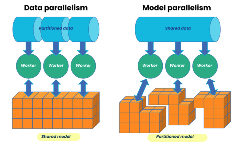
Data Parallelism

• Multiple workers (GPUs), but only one model to train.
  • All GPUs have a version of the model and optimizer states.
  • Split data up such that each worker sees a different set of data.
  • Once a forward pass is complete for all workers, each model computes a gradient.
  • Gradients are averaged and then model is updated.
• Data Parallel using AllReduce
  • Computation happens on all workers
  • Gradients are transferred directly to workers using AllReduce.
  • Model is transferred to all workers with AllReduce
• Synchronous Data Parallelism
  • All workers wait until all other GPUs finish calculating gradients and then average them to update the shared model.
  • Synchronous is more often used with strong devices with powerful communication links.
• Asynchronous Data Parallelism
  • Workers are not synchronized, instead updates happen asynchronously.
• Data Parallel Pitfalls
  • Keep the local batch size constant and scale the global batch size, but you must also change hyperparameters such as the learning rate because you are using a much larger effective batch size.
    
    

Model Parallelism

• If our model won’t fit on one GPU, we can use model parallelism.
• Split the model across worker GPUs and it can be used to make batches bigger.
  
  

• DataParallel (DP) vs. DistributedDataParallel (DDP)
  • PyTorch’s DataParallel
    • Single process but multi-threaded
    • Works on only a single machine
    • Usually slower that DistributedDataParallel
    • Does not support model parallel training
  • PyTorch’s DistributedDataParallel
    • Works on 1 or more machines
    • Usually much faster than DataParallel
    • Supports model parallel, data parallel, FSDP, and other paradigms
  • Data Parallel performs three GPU transfers for every batch:
    1. Copy model to device
    2. Copy data to device
    3. Copy outputs of each device back to master
  • Distributed data parallel (DDP) performs 1 transfer to sync gradients. This makes DDP much faster!
    
    
    

Fully Sharded Data Parallel (FSDP)

If we want to train a 1.5B GPT-2 model, it will just require 3GB of memory for its weights… but if we were to use a single GPU we would need 32GB of VRAM in FP16. Why?

• The rest of the memory is consumed by optimizer states, storing gradients, and storing activations.
• Temporary buffers used for distributed communication also consume memory.
• Moreover, we have memory fragmentation issues to deal with.
  
  
• Sharding: to partition data or tasks into smaller, more manageable pieces (called shards) and distribute them across multiple servers, databases, or devices.
  • Sharding is a technique to greatly reduce peak memory usage on your GPUs when using distributed training.
  • It is like a hybrid of model and data parallel and involves splitting the parameters across devices.
    
    
• FSDP (Fully Sharded Data Parallel): an extension of the data parallel training paradigm and is part of the FairScale library, developed by Facebook AI, to allow the training of large models by breaking down and distributing both the model parameters and gradients across multiple GPUs, reducing the overall memory footprint and making efficient use of hardware.
  • FSDP shards a model’s parameters, gradients, and optimizer states across data parallel workers, while maintaining the simplicity of data parallelism.
  • It is a hybrid of model parallelism, data parallelism, with a lot of additional optimizations.
    
    
• Data Parallel vs FSDP
  • Data parallel training: Each worker processes a separate batch and gradients are summed across workers using an all-reduce operation.
    • This means each model keeps a copy of the weights and the optimizer states, so the amount of VRAM for model and optimizer is 2-3x the size of the model.
  • FSDP: A subset of model parameters, gradients, and optimizers are kept on each GPU. It is an optimization based approach.
    
    
    

There are many ways to use distributed processing. Most combine it with other techniques, (e.g., AMP.) In general,

• If the model fits on one GPU and you can use sufficiently large batches, use data parallel training.
• Model parallel and sharding should be used if you have large models.
• Use data parallel if models are less than 200M parameters
  • May not always hold depending on memory needed for forward pass, e.g., semantic
  • segmentation can use far more than classification.
• Use model parallel approaches like DeepSpeed, FSDP, etc. if models are over 500M parameters.