Day89 ML Review - Ensemble Method (5)

October 11, 2024 7 minute read

Revisiting Ensemble Method, Random Forest, and XGBoost

Source: Analytics Vidhya - Ensemble Learning Methods

As we further examine the Ensemble Method in machine learning, we find it integrates several machine learning models. One challenge in this field is that individual models often yield subpar results, and they are known as weak learners. To address this issue of low prediction accuracy, we merge multiple models to develop a more effective one.

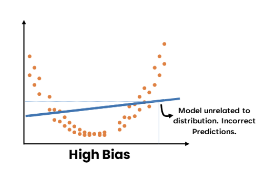
As mentioned in earlier posts, a model with high bias or high variance leads to inaccurate predictions.

A high-bias model arises when the data isn’t sufficiently learned or linked to its distribution. (Bias reflects how much a model’s prediction deviates from the target value based on training data. It results from simplifying assumptions in the model, making the target functions easier to approximate.)
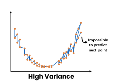
High variance, often overfitting, happens when a machine learning model or statistical algorithm pays too much attention to particular patterns in the training data, leading to poor generalization on new, unseen data. (Variance measures how much a random variable diverges from its expected value, using a single training set to evaluate prediction variability across various training sets.)

Ensemble learning aims to reduce the bias if we have a weak model with high bias and low variance.

Source: IBM: What is Random Forest?

Random Forest

The random forest algorithm builds on the bagging method by incorporating both bagging and feature randomness, resulting in a diverse collection of uncorrelated decision trees. Feature randomness allows for the creation of a random selection of features, which helps maintain low correlation between the decision trees.

How it works

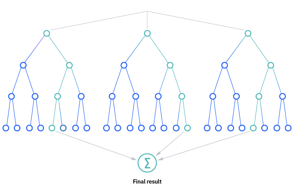
Image Source: [IBM: What is Random Forest?]

Random forest algorithms need three key hyperparameters before training: node size, tree count, and sampled features. After setting these, the classifier can tackle regression and classification tasks.

The random forest algorithm comprises multiple decision trees, where each tree is created from a bootstrap sample—a data sample taken from the training set with replacement.

The method of determining predictions depends on the type of problem. In regression tasks, the predictions from individual decision trees are averaged, while in classification tasks, the most frequent categorical variable is chosen through a majority vote. Then, the out-of-bag (OOB) sample is utilized for cross-validation to finalize the prediction.

Key Benefits

Reduced risk of overfitting: Decision trees are prone to overfitting because they often closely fit all training samples. In contrast, with a sufficient number of trees in a random forest, the classifier avoids overfitting. Overall variance and prediction error are reduced by averaging the predictions from uncorrelated trees.
Provides flexibility: Random forests are favored by data scientists because they accurately handle both regression and classification tasks. Additionally, feature bagging makes the random forest classifier effective for estimating missing values while retaining accuracy even when some data is absent.
Easy to determine feature importance: Random forests simplify the evaluation of variable importance or their contribution to the model. Several methods can assess feature importance, including Gini importance and mean decrease in impurity (MDI), which measure the drop in model accuracy when a variable is excluded. Another significant method, permutation importance or mean decrease accuracy (MDA), gauges the average accuracy loss by randomly permuting feature values in out-of-bag samples.

Key Challenges

Time-intensive procedure: Although random forest algorithms can manage large datasets for more precise predictions, they tend to be slow since they compute data for each decision tree.
Heightened resource requirements: Random forests necessitate additional resources for storing larger datasets.
Increased complexity: A single decision tree’s prediction is more accessible to interpret compared to a forest of trees.

Check my post (Day 64-65) to see the code implementation.

Explanation Source: Analytics Vidhya - End-to-End guide to Understanding the Math behind XGBoost

XGBoost

XGBoost is a machine learning algorithm that falls under the category of ensemble learning, focusing specifically on the gradient-boosting framework. It uses decision trees as its foundational learners and incorporates regularization techniques to improve model generalization. XGBoost is recognized for its computational efficiency, fast processing, valuable feature importance analysis, and effective handling of missing values. It is widely preferred for various applications, including regression, classification, and ranking.

XGBoost creates a predictive model by iteratively aggregating predictions from multiple individual models, typically decision trees. The algorithm sequentially introduces weak learners, with each new learner aimed at correcting the previous ones’ errors. It employs a gradient descent optimization method to minimize a specified loss function during training.

Notable features of the XGBoost algorithm are its capacity to manage intricate data relationships, regularization techniques to avoid overfitting, and the implementation of parallel processing for enhanced computational efficiency.

Mathematics Explanation

Let’s explore Gradient Boosting within the ensemble method. XGBoost constructs trees one after another, optimizing a regularized objective function by leveraging both gradients and second-order Hessians. It allocates weights to leaf nodes, assesses splits according to their gain, and prunes trees to prevent overfitting.

Step 1: Define the Objective Function

The goal of XGBoost is to minimize the objective function, which combines the loss function and a regularization term to prevent overfitting:

$\mathcal{L}(\phi) = \sum_{i=1}^{n} L(y_i, \hat{y}_i) + \sum_{k=1}^{T} \Omega(f_k)$

Where:

$n$: Number of data points (samples).
$T$: Total number of trees.
$L(yi,\hat{y^i})$: Loss function measuring how close the predictions $\hat{y^i}$ are to the true values $y_i$. Examples include Mean Squared Error (MSE) for regression or Log Loss for classification.
$\Omega(f_k)$: Regularization term to penalize model complexity.

Step 2: Use Taylor Expansion to Approximate the Objective

XGBoost uses a second-order Taylor expansion to efficiently approximate the objective function around the current predictions. Give the loss function above, and expand it around the prediction $\hat{y_i}^{(t)}$

$L(y_i, \hat{y}_i + f_t(x_i)) \approx L(y_i, \hat{y}_i) + g_i f_t(x_i) + \frac{1}{2} h_i f_t(x_i)^2$

Where:

$g_i = \frac{\partial L(y_i, \hat{y}_i)}{\partial \hat{y}_i}$ is the first-order gradient (residual).
$h_i = \frac{\partial^2 L(y_i, \hat{y}_i)}{\partial \hat{y}_i^2}$ is the second-order gradient (curvature).

Thus, the objective function for step $t$ becomes as follows. This approximation makes optimization faster since it use both gradients and Hessians.

$\mathcal{L}^{(t)} = \sum_{j=1}^{J} \left[ \sum_{i \in I_j} \left( g_i w_j + \frac{1}{2} h_i w_j^2 \right) \right] + \gamma J + \frac{1}{2} \lambda \sum_{j=1}^{J} w_j^2$

Step 3: Define the Structure of Decision Trees

Each tree makes predictions by assigning an input $x_i$ to a leaf node. Assume the tree has $j$ leaf nodes.

The model’s prediction for a sample is the weight of the leaf node that the sample is assigned to. Let $I_j$ be the set of samples assigned to the $j$-th leaf node.

Step 4: Optimize Leaf Weights

Each tree has several leaf nodes, and the optimal weight for each leaf is calculated by minimizing the following function.

$\mathcal{L}^{(t)} = \sum_{j=1}^{J} \left[ \sum_{i \in I_j} \left( g_i w_j + \frac{1}{2} h_i w_j^2 \right) \right] + \gamma J + \frac{1}{2} \lambda \sum_{j=1}^{J} w_j^2$

To find the optimal weight $w_j^*$ for each leaf node, we set the derivative of the objective function with respect to $w_j$to zero:

$\frac{\partial \mathcal{L}}{\partial w_j} = \sum_{i \in I_j} \left( g_i + h_i w_j \right) + \lambda w_j = 0$

Solving for $w_j$, we get:

$w_j^* = -\frac{\sum_{i \in I_j} g_i}{\sum_{i \in I_j} h_i + \lambda}$

This is the optimal weight for each leaf, balancing between the gradients and the regularization term $\lambda$.

Step 5: Calculate the Gain for Splitting Nodes

The split gain is the improvement in the objective when a node is split into two child nodes (left and right). For a given split:

$\text{Gain} = \frac{1}{2} \left( \frac{G_L^2}{H_L + \lambda} + \frac{G_R^2}{H_R + \lambda} - \frac{(G_L + G_R)^2}{H_L + H_R + \lambda} \right) - \gamma$

$ G_L $ and $ H_L $: Sum of gradients and Hessians for the left child.
$ G_R $ and $ H_R $: Sum of gradients and Hessians for the right child.
$\gamma $: Regularization penalty for adding new leaves.

Step 6: Make Predictions Using the Final Model

After constructing $T$ trees, the final prediction for a given input $x_i$ is the sum of the predictions from all trees:

$\hat{y}_i = \sum_{t=1}^{T} f_t(x_i)$

For classification tasks, the predictions can be transformed using the softmax or sigmoid functions to get probabilities.

Comparison of XGBoost and Random Forest

Feature	XGBoost	Random Forest
Description	Improves errors from previous trees	Builds trees independently
Algorithm Type	Boosting	Bagging
Handling of Weak Learners	Corrects errors sequentially	Combines predictions of independently built trees
Regularization	Uses L1 and L2 regularization to prevent overfitting	Usually doen’t employ regularization techniques
Performance	Often performs better on structured data but needs more tuning	Simpler and less prone to overfitting

Share on

Twitter Facebook LinkedIn

Wonha Leah Shin