Day90 Deep Learning Lecture Review - Background Knowledges

October 12, 2024 7 minute read

HW0: Softmax Properties, PyTorch Lightning, and DataLoader

Softmax Properties

Definition

The softmax function is a typical activation function used in machine learning, particularly in the final layer of a neural network for classification tasks. It converts raw model outputs (often called logits) into probabilities that sum to 1. Below, I’ll describe its properties and why they are helpful.

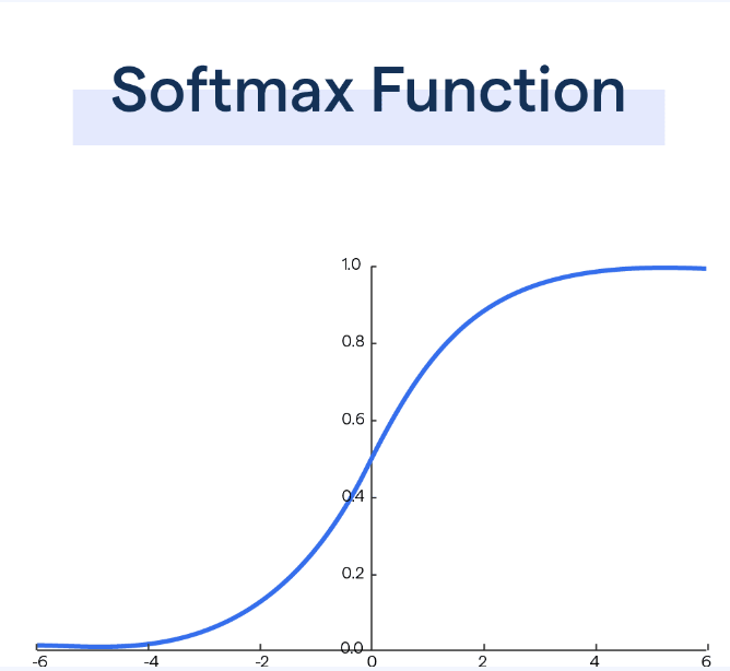
Partial source of contents: [Wikipedia-Softmax Function]

Image Source: [BotPenguin : Softmax Function]

Main Properties of Softmax

1. Output Values are Probabilities

The output values of the softmax function are in the range $(0,1)$, making them interpretable as probabilities.
Each output represents the probability of the input belonging to a particular class.

2. Sum to One

The sum of the softmax outputs over all classes is always equal to 1:

\[\sum^K_{i=1} \text{softmax}(z_i) = 1\]

This property ensures that the output form a valid probability distribution.

3. Exponentiation Emphasizes Differences

The use of the exponential function $e^{z_i}$ makes larger scores even larger and smaller scores even smaller, which magnifies the difference between logits.

4. Sensitive to Scale

Softmax can be sensitive to the scale of logits. If the values are very large, the exponentiation can cause numerical instability. To address this, it’s common to subtract the maximum value of the logits from all the logits before applying softmax (this doesn’t affect the output since it’s the same for all terms):

\[\text{softmax}(z_i) = \frac{e^{zi}-z_{max}}{\sum_{j=1}^K e^{z_j-z_{max}}}\]

5. Class Separation

The class with the highest value tends to dominate the probabilities because of the exponential function. If one of the input scores is much larger than the others, softmax will assign a high probability to that class and very low probabilities to the others.

6. Cross-Entropy Compatibility

Softmax is often used with the cross-entropy loss function in classifiaction tasks. This paring works well because cross-entropy measures the difference between the predicted probability distribution (produced by softmax) and the true distribution (typically one-hot encoded).

7. Practical Usage in Machine Learning

Classification Tasks: Softmax is primarily used for multi-class classification problemd where each input should be assigned to exactly one of the $K$ classes.
Final Output Layer: In neural networks, softmax is typically used in the final layer to produce a probability distribution that can be used to determine which class an input belongs to.

Assignment Review

In this assignment, I should explore a fundamental property of the softmax function. The goal was to prove that the softmax function is invariant to constant offsets in its output.

This means that if you add the same constant value to each element of the input vector, the ouput probabilities produced by somftmax remain unchanged. This property is crucial for ensuring numerical stability when training deep learning models, particularly when logits (model outputs before applying softmax) become very large or very small. By leveraging this property, we can prevent overflow and underflow issues, making computations more efficient and stable.

Additionally, I discussed why this property matters in practical neural network implementations. The constant-offset invariance allows us to subtract the maximum logit value from all logits, keeping calculations manageable and stable during training. This trick is especially important for ensuring stable cross-entropy loss calculations and maintaining effective gradient-based optimization.

Proving Softmax Invariance to Constant Offsets

1. Rewrite the softmax function

Consider the input $\mathbf{a} + c\mathbf{1}$, where $c\mathbf{1}$ is a vector of length $K$ with each element equal to the constant $c$.
The new softmax function becomes:
$\text{softmax}(\mathbf{a} + c\mathbf{1}) = \frac{\exp(a_i + c)}{\sum_{j=1}^K \exp(a_j + c)}$

2. Simplify

The exponential function distributes over addition, which gives:
$\text{exp}(a_i+c)= \text{exp}(a_i) \cdot \text{exp}(c)$

3. Factor out $\text{exp}(c)$:

Both the numerator and the denominator contain the term $\exp(c)$, which can be factored out and canceled:
$ \text{softmax}(\mathbf{a} + c\mathbf{1}) = \frac{\exp(a_i) \cdot \exp(c)}{\sum_{j=1}^K \exp(a_j) \cdot \exp(c)} = \frac{\exp(a_i)}{\sum_{j=1}^K \exp(a_j)}$
After cancellation, the resulting expression is the same as the original softmax function:
$ \text{softmax}(\mathbf{a} + c\mathbf{1}) = \text{softmax}(\mathbf{a})$

This shows that adding a constant offset to every element of the input vector does not change the output of the softmax function.

Source: [PyTorch Lightning Documentation]

PyTorch Lightning

PyTorch Lightning is a high-level framework built on top of PyTorch that simplifies the process of building and training deep learning models. It abstracts away much of boilerplate code involved in training, validation, and logging, allowing developers to focus more on the model logic and experimentation.

PyTorch Lightning is designed to make models more scalable, readable, and reproductiable by providing a structurred approach to PyTorch code.

How to Use PyTorch Lightning

Install PyTorch Lightning
```
pip install pytorch-lightning
```

Define The Model: In PyTorch Lightning, we define the model by subclassing LightningModule. We will need to implement the following key methods:

__init__: Define the layers of the model
forward(): Define the forward pass
training_step(): Define a single training step
configure_optimizers(): Define the optimizers and learning rate schedulers

import pytorch_lightning as pl
import torch
from torch import nn
   
class MyModel(pl.LightningModule):
  def __init__(self):
    super().__init__()
    self.layer = nn.Linear(28*28, 10)
       
  def forward(self, x):
    return self.layer(x)
     
  def training_step(self, batch, batch_idx):
    x, y = batch
    y_hat = self(x)
    loss = nn.functional.cross_entropy(y_hat, y)
    return loss
     
  def configure_optimizers(self):
    optimizer = torch.optim.Adam(self.parameters(), lr=1e-3)
    return optimizer

Train the Model: Use the Trainer class to train your model.

model = MyModel()
trainer = pl.Trainer(max_epochs=5)
trainer.fit(model, train_dataloader, val_dataloader)

Benefits:
- Simplifies Training Loops: Automatically handles the training loop, validation, and logging.
- Scalability: Easily scale the code to multiple GPUs, TPUs, or even clusters.
- Modular Design: Separates concerns of training, evaluation, and model architecture, making the code more readable and maintainable.

Feedforward Fully-Connected Networks for Iris Dataset Classification

For this assignment, I worked on implementing feedforward fully-connected neural networks using PyTorch and PyTorch Lightning to classify given Iris dataset. The dataset consists of three classes, and each row contains a label and two features.

Data Preparation: Using the datasets I have, each row represents a data instance labeled 1, 2, or 3, with two features. After loading the dataset, I normalized it by subtracting the mean and then split it into training and test sets.
Neural Network Architectures
- Linear Model: The first neural network was a basic linear classifier consisting solely of an output layer, depicted as a $2 \times 3$ matrix. Essentially, it performed a linear transformation with an added bias term.
- Nonlinear Model: In contrast, the second model featured a hidden layer containing 5 units, using ReLU activation to function as a nonlinear classifier.
Training Setup: Both models utilized the AdamW optimizer and CrossEntropyLoss over 1000 epochs. Multiple runs were conducted with various random initializations to avoid poor local optima.

Code Snippets and Explanations

Data Loading and Normalization

from sklearn.preprocessing import StandardScaler
import torch
import numpy as np
   
# Load the dataset
train_data = np.loadtxt('iris-train.txt', delimiter=' ')
test_data = np.loadtxt('iris-test.txt', delimiter=' ')
   
# Split data into features and labels
X_train, y_train = train_data[:, 1:], train_data[:, 0].astype(int) - 1
X_test, y_test = test_data[:, 1:], test_data[:, 0].astype(int)-1
   
# Normalize the Data
scaler = StandardScaler()
X_train = scaler.fit_transform(X_train)
X_test = scaler.transform(X_test)

train_data[:, 1:] selects all rows and all columns expect the first, which represents the features (input variables) of the dataset.
train_data[:, 0].astype(int) - 1 selects the labels (target variable) from the first column and converrts them to integers. The subtraction by 1 ensures that the labels are zero-indexed, which is common in machine learning frameworks like PyTorch, where class indices start from 0 instead of 1.

Linear and Nonlinear Models

Linear Model

import torch.nn as nn
import pytorch_lightning as pl
  
class LinearModel(pl.LightningModule):
  def __init__(self):
    super(LinearModel, self).__init__()
    self.linear = nn.Linear(2,3)
    self.loss_fn = nn.CrossEntropyLoss()
      
  def forward(self, x):
    return self.linear(x)
    
  def training_step(self, batch, batch_idx):
    x, y = batch
    y_hat = self.forward(x)
    loss = self.loss_fn(y_hat, y)
    return loss
    
  def configure_optimizers(self):
    return torch.optim.AdamW(self.parameters(), lr=0.01)

Nonlinear Model:

class NonLinearModel(pl.LightningModule):
  def __init__(self):
    super(NonLinearModel, self).__init__()
    self.hidden = nn.Linear(2, 5)
    self.output = nn.Linear(5, 3)
    self.relu = nn.ReLU()
    self.loss_fn = nn.CrossEntropyLoss()
     
  def forward(self, x):
    x = self.relu(self.hidden(x))
    return self.output(x)
    
  def training_step(self, batch, batch_idx):
    x, y = batch
    y_hat = self.forward(x)
    loss = self.loss_fn(y_hat, y)
    return loss
    
  def configure_optimizers(self):
    return torch.optim.AdamW(self.parameters(), lr=0.01)

3. Training the Models

Training both models

from torch.utils.data import DataLoader, TensorDataset
  
# Convert data to PyTorch tensors
X_train_tensor = torch.tensor(X_train, dtype=torch.float32)
y_train_tensor = torch.tensor(y_train, dtype=torch.long)
  
# Create DataLoader
train_loader = DataLoader(TensorDataset(X_train_tensor, y_train_tensor), 
                          batch_size=16, shuffle=True)
  
# Train the models
linear_model = LinearModel()
nonlinear_model = NonLinearModel()
trainer = pl.Trainer(max_epochs=1000)
trainer.fit(linear_model, train_loader)
trainer.fit(nonlinear_model, train_loader)

Convert Data to Tensors:
- X_train_tensor = torch.tensor(X_train, dtype=torch.float32) and y_train_tensor = torch.tensor(y_train, dtype=torch.long):
  - Using the line above, we convert the training feature matrix (X_train) and labels(y_train) into PyTorch tensors, which are the data structure PyTorch uses for efficient computation, similar to NumPy arrays but with the added functionality for GPU acceleration.
  - dtype=torch.float32 is used for input features, while dtype=torch.long is used for labels, which is required for classification.

Side Note: DataLoader

A DataLoader in PyTorch is a utility that wraps a dataset and provides an easy way to iterate over the data in mini-batches. it is commonly used during model training and evaluation to handle data loading efficiently.

Source: [PyTorch Tutorial - Datasets & DataLoaders]

Why do we use DataLoader?

Efficiency: It handles loading data in a way that keeps the GPU/CPU busy, avoiding the bottleneck of waiting for new data.
Batch Management: Automatically splits data into mini-batches, which is essential for training with gradient-based optimizers.
Data Shuffling: Shuffling the data is crucial for preventing overfitting and ensuring that the model generalizes well.
Flexibility: DataLoader can work with any kind of dataset, such as images, text, or tabular data, making it versatile for a wide variety of deep learning tasks.

Share on

Twitter Facebook LinkedIn

Wonha Leah Shin