Day91 Deep Learning Lecture Review - Optimizing Hyperparameters

📚 The Start of Recording TIL Summer ‘24 : Why Did I Start This Project? 🚀

🔔 Don't Miss: Continous Records of TIL '25 (Still On-Going!) 🌟

✨ A New Chapter in TIL '25: Reflecting, Growing, and Moving Forward 📖

Weights & Biases (W&B) for Monitoring and Fine-Tuning ResNet-18 and Post-Training Evaluations (Dying ReLU, Brightness Robustness)

I explored hyperparameter tuning, network fine-tuning, and monitoring model performance with Weights and Biases (W&B) in this latest assignment. The primary goal was to train ResNet-18 for image classification on the Oxford-IIIT Pet Dataset while optimizing different model parameters. Here’s a summary of my workflow, the results, and the insights I gained throughout the process.

W&B for Training Monitoring

Training neural networks involves balancing various model architectures, hyperparameters, and optimization strategies. To make these decisions effectively, monitoring the training process and understanding the impact of changes on model performance is essential. I used W&B to log metrics such as training loss, validation accuracy, test accuracy, and other performance indicators.

*I utilized Google Colab since W&B does not cater to some Mac environment users.

1. Dataset Preparation: I was provided the Oxford-IIIT Pet Dataset by resizing the images (as required by ResNet-18) and applying normalization. This setup aligns with the requirements for training ResNet-18, which expects input data similar to the ImageNet Dataset.

2. Implementing W&B Logging: I integrated W&B into the training script by logging:

   • Training loss and learning rate after each mini-batch.
   • Validation loss and accuracy after each epoch.
   • Final test loss and accuracy.

   import wandb
   wandb.init(project="resnet-oxford-pets")
      
   # Inside of training loop
   # Log training metrics to W&B
   wandb.log({
     'train_loss': loss.item(),
     'learning_rate': optimizer.param_groups[0]['lr'],
     'seen_examples': seen_examples,
     'global_step': global_step
             })
      
   if global_step % batch_steps == 0:
     val_acc, val_loss = evaluate(model, val_loader, device)
      
        
   # Log validation metrics to W&B
   wandb.log({
     'val_loss': val_loss,
     'val_accuracy': val_acc,
     'epoch': epoch,
     'seen_examples': seen_examples
   })
      
   if best_val_loss > val_loss:
     best_val_loss = val_loss
     os.makedirs(os.path.join(save_dir, f'{run_name}_{rid}'), exist_ok=True)
     state_dict = model.state_dict()
     torch.save(state_dict, os.path.join(save_dir, f'{run_name}_{rid}', 'checkpoint.pth'))
     print(f'Checkpoint at step {global_step} saved!')
      
      
   # Log metrics to W&B
   wandb.log({
     'loss (batch)': loss.item(),
     'global_step': global_step,
     'seen_examples': seen_examples
   })
   

   
   
   

3. Result- Observations

   • Training Loss: The training loss consistently decreased, indicating that the model learned from the data effectively.
   • Validation Loss: In contrast to the training loss, the validation loss increased over time, suggesting that the model overfitted the training data. This highlights the importance of validation monitoring to maintain generalizability.
   • Test Accuracy: The final test accuracy was relatively low, around 2%, indicating poor generalization. This led me to re-evaluate the model’s settings and consider additional techniques.

Tuning Hyperparameters

I concentrated on tuning hyperparameters, particularly the learning rate during this phase, utilizing a W&B sweep. The goal was to identify the best settings for enhancing the model’s performance.

Learning Rate Tuning

• I ran multiple experiments using learning rates: $1e-2$, $1e-3$, $1e-4$, $1e-5$, with the default being $1e-3$

  sweep_config = {
    'method' : 'grid',
    'parameters' : {
      'learning_rate': {
        'values': [1e-2, 1e-3, 1e-4, 1e-5]
      }
    }
  }
  sweep_id = wandb.sweep(sweep_config, project="resnet-oxford-pets")
  wandb.agent(sweep_id, function=train)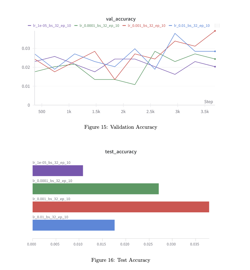
  

  
  
  

• Key Insights

  • The learning rate of $1e-3$ consistently showed the best convergence and generalization performance, leading to lower training loss and higher validation and test accuracy.

  • Higher learning rates led to oscillation without convergence, whereas very low rates caused slow learning and the risk of underfitting.

  • Charts comparing the learning rate impacts demonstrated that 0.001 was optimal, balancing efficient learning and model stability.

Learning Rate Scheduler with OneCycleLR

To improve training efficiency and convergence, I implemented the OneCycleLR scheduler. This scheduler dynamically adjusts the learning rate, starting with a low value, increasing it to a peak, and gradually reducing it.

from torch.optim.lr_scheduler import OneCycleLR

optimizer = torch.optim.Adam(model.parameters(), lr=1e-3)
scheduler = OneCycleLR(optimizer, max_lr=1e-2, steps_per_epoch = len(train_loader),
                      epochs = num_epochs)


# In the Train loop
if use_scheduler:scheduler = lr_scheduler.OneCycleLR(
  optimizer,
  max_lr=kwargs.get('max_lr', 0.01),
  total_steps=kwargs.get('total_steps', 1000),
  pct_start=kwargs.get('pct_start', 0.3),
  anneal_strategy=kwargs.get('anneal_strategy', 'linear'), 
  final_div_factor=kwargs.get('final_div_factor', 10)
)
else:
  scheduler = None
  return scheduler

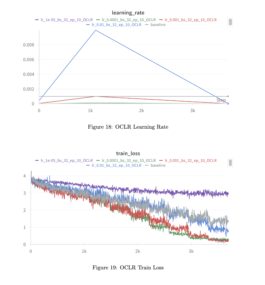
• Results with OneCycleLR
  • The training process with OneCycleLR showed faster convergence compared to the baseline with a static learning rate. The model benefited from higher initial leraning rates to explore the parameter spze, followed by reduced rates for finer adjustments.
  • However, validation accuracy fluctuated more than the baseline, highlighting that a dynamic learning rate can sometimes introduce instability but ultimately leads to better test accuracy.

Fine-Tuning a Pretrained ResNet-18

Lastly, I fine-tuned a ResNet-18 model pre-trained on ImageNet. Fine-tuning leverages the pre-learned features and adapts them to the specific task, in this case, classifying pet images.

import torchvision.models as models

# Load a pretrained ResNet-18 model
model = models.resnet18(pretrained=True)

# modify the final layer to match the number of classes in the pet dataset
model.fc = nn.Linear(model.fc.in_features, num_classes)

# Freeze all layers except the final one
for param in model.parameters():
  param.requires_grad = False
for param in model.fc.parameters():
  param.requires_grad = True

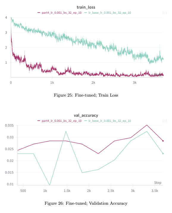
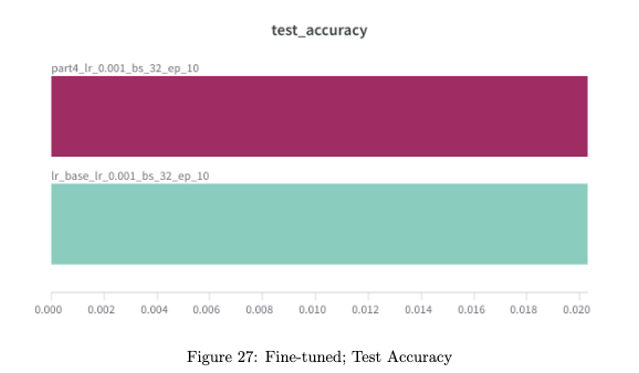
• Comparison with Training from Scratch
  • Training Loss: The pre-trained model showed significantly faster convergence, reducing the loss in fewer epochs compared to the baseline model.
  • Validation and Test Accuracy: The fine-tuned model also outperformed the baseline in validation and test accuracy, underscoring the benefit of using transfer learning to quickly adappt strong feature representations from large datasets like ImageNet.

Model Testing

Pre-Train Testing

Pre-Train Test: Conducted before training, these tests identify potential issues in the model’s architecture, data preprocessing, or other components, preventing wasted resources on flawed training.

• Data Leakage Check: I compared image hashes to check for potential data leakage between training, validation, and test sets.
  • Observation: There was no overlap between training and validation, but 5,000 images overlapped between training and test sets. This indicates a severe data leakage problem, which could lead to inflated test performance.
  • Solution: Re-split the dataset to eliminate overlap, ensuring each set is unique to maintain fair evaluation.
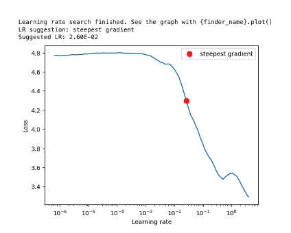
• Learning Rate Tuning: I used a learning rate range test to identify the optimal learning rate for training the model. The graph suggested an optimal learning rate of around 0.026, at which point the loss decreased rapidly.
  • Analysis: An optimal learning rate is crucial for efficient training and stability. A value too high leads to unstable training, while a low value causes slow convergence.

• Model Architecture Check: to verify that the model’s output shape matches the label format;
  • Initialized the model and identified an incorrect output shape of $[1, 128]$ instead of the expected $[1, 10]$.
  • Modified the final fully connected layer to output the correct number of features (10).
• Gradient Descent Validation: to verify that all the models’ trainable parameters are updated after a single gradient step on a batch of data.
  • Detected that parameters in the downsample layers were not receiving gradients.
  • Implemented a function to check for missing gradients and reviewed the architecture for necessary adjustments.
    
    

Post Train Testing

I examined the trained model’s robustness by focusing on post-training evaluations, particularly detecting common issues such as Dying ReLU and assessing its resilience to brightness variations**. Below are the key areas and findings.

• Dying ReLU Examination: Dying ReLU occurs when a ReLU activation function consistently outputs zero, effectively making a neuron non-contributive. This can lead to ineffective learning since such “dead” neurons no longer help the model learn meaningful features.

  • Approach: I registered hooks on the ReLU layers in my model to capture their outputs during a forward pass through the test dataset.

  • Observation: After analyzing the ReLU activations, I found slightly significant Dying ReLU neurons in my trained model.

    # Hook to store ReLU outputs
    relu_outputs = []
        
    def relu_hook(module, input, output):
        relu_outputs.append(output.clone().detach())
        
    # Register hooks on ReLU activations
    for layer in model.modules():
        if isinstance(layer, torch.nn.ReLU):
            layer.register_forward_hook(relu_hook)
        
    # Forward pass to check activations
    with torch.no_grad():
        for images, labels in test_loader:
            _ = model(images)
        
    # Analyzing the collected ReLU outputs
    dying_relu_neurons = sum(torch.sum(relu_output == 0).item() for relu_output in relu_outputs)
    print(f"Dying ReLU neurons: {dying_relu_neurons} detected.")
    

• **Model Robustness to Brightness Changes: To further evaluate the model’s robustness, I tested its ability to classify images under different brightness levels.

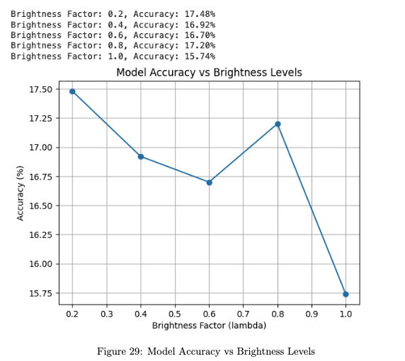
  • Brightness Factor Evaluation: I adjusted the brightness of the test images by multiplying pixel values with a factor λ, ranging from 0.2 to 1.0 in increments of 0.2. This allowed me to observe how the model performed across varying lighting conditions.

  • Results:

    • Highest Accuracy at Low Brightness: The model performed best at a low brightness factor of λ = 0.2, achieving an accuracy of around 17.48%.

    • Performance Degradation: As brightness increased, accuracy dropped, with the lowest accuracy recorded at λ = 1.0 (original brightness level), indicating that the model was not well-optimized for well-lit images

      # Adjust brightness levels and evaluate
      brightness_levels = [0.2, 0.4, 0.6, 0.8, 1.0]
      for level in brightness_levels:
          transformed_images = apply_brightness_factor(test_images, level)
          accuracy = evaluate_model(model, transformed_images, labels)
          print(f"Accuracy at brightness level {level}: {accuracy:.2f}%")
      

• Normalization Mismatch: An analysis was conducted to assess normalization differences between the training and test sets.

• Calculated vs. Expected Statistics: The test set’s mean and standard deviation showed significant deviation from the expected values. For example, the calculated mean was close to zero, while the expected values were approximately 0.49, 0.48, and 0.44 for the RGB channels.

• Impact: This inconsistency in normalization may lead to the model encountering inputs that fall outside the range it was trained on, which could result in poor generalization and incorrect predictions during inference.

Throughout the entire journey of processing whole procedures, from fine-tuning a model to executing post-tests, I gained a profound understanding of several critical aspects of machine learning. The significance of model validation became abundantly clear, showcasing how essential it is to ensure a model’s performance is robust and reliable.