Day92 Deep Learning Lecture Review - Fine-Tuning Models (1)

📚 The Start of Recording TIL Summer ‘24 : Why Did I Start This Project? 🚀

🔔 Don't Miss: Continous Records of TIL '25 (Still On-Going!) 🌟

✨ A New Chapter in TIL '25: Reflecting, Growing, and Moving Forward 📖

HW2: Understanding of LoRA and Pre-trained Model Embeddings (ResNet+SBERT) for Visual Question Answering (VQA)

Recently, I conducted several experiments with LoRA (Low-Rank Adaptation), an innovative approach to efficiently fine-tune large pre-trained language models for sentiment analysis and compare it to traditional fine-tuning methods. Here, I want to share the insights I discovered and the key lessons I learned through this experience.

Understanding LoRA

LoRA fine-tunes large language models in a computationally demanding manner, requiring adjustments to all model parameters. However, LoRA cleverly addresses this issue by modifying only the **low-rank components of a weight matrix instead of every parameter. I fine-tuned the roberta-base model for sentiment classification using the TweetEval dataset in my experiment. First, I applied standard fine-tuning, followed by LoRA, to evaluate the efficiency and performance of both approaches.

Fine-tuning large language models is often computationally costly because all model parameters must be updated. I discovered that LoRA offers a more efficient solution by only modifying low-rank weight matrix components while keeping most of the original model unchanged. This approach significantly lowers the number of trainable parameters, reducing computational expenses. In particular, LoRA enhances weight matrices by incorporating low-rank updates, enabling practical training without significantly compromising performance.

In my experiments, I analyzed the impact of LoRA on both computational efficiency and model accuracy. I also explored where LoRA could be integrated into Transformer architectures. I learned that LoRA is commonly applied to the query and value projection matrices in the self-attention mechanism, which allows it to efficiently adapt the model while maintaining the integrity of the original pre-trained weights. This approach was insightful because it showcased leveraging low-rank adaptations for efficient fine-tuning.

Comparing Standard Fine-Tuning and LoRA

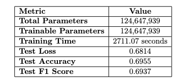
To understand the impact of LoRA in a practical setting, I fine-tuned the roberta-base model on the TweetEval Sentiment dataset using both standard fine-tuning and LoRA. I updated all model parameters for the standard fine-tuning, resulting in approximately 124.6 million trainable parameters. The training took over 2700 seconds, and the test accuracy was 0.6955. This gave me a baseline for comparison.

The code snippet for standard fine-tuning using Hugging Face’s Transformers library:

from transformers import robertaForSequenceClassification, Trainer, TrainingArguments
from datasets import load_dataset

# Load dataset and model
dataset = load_dataset("tweet_eval", name="sentiment")
model = RobertaForSequenceClassification.from_pretrained("roberta-base", num_labels=3)

# Training arguments
training_args = TrainingArguments(
		output_dir="./results",
    evaluation_strategy="epoch",
    num_train_epochs=1,
    per_device_train_batch_size=16,
    per_device_eval_batch_size=16,
    logging_dir="./logs",
    logging_steps=10,
    save_total_limit=2
)

trainer = Trainer(
    model=model,
    args=training_args,
    train_dataset=dataset["train"],
    eval_dataset=dataset["validation"]
)

# Train model
trainer.train()

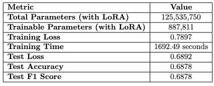
Next, I implemented LoRA using the Hugging Face PEFT library. By applying LoRA, I reduced the trainable parameters as below.

The code snippet for fine-tuning with LoRA using PEFT:

from peft import LoraConfig, get_peft_model, TaskType

# Configure LoRA using PEFT
lora_config = LoraConfig(
    r=8,  # Rank
    inference_mode=False,  # Training mode
    task_type=TaskType.SEQ_CLS  # Sequence classification
)

# Apply LoRA to the model
model = get_peft_model(model, lora_config)

# Training arguments (same as above)
trainer = Trainer(
    model=model,
    args=training_args,
    train_dataset=dataset["train"],
    eval_dataset=dataset["validation"]
)

# Train model with LoRA
trainer.train()

I gained a critical insight from this comparison: LoRA can be particularly beneficial in resource-constrained environments with limited memory and computational power. It offers an effective way to fine-tune models without requiring the full computational load of standard fine-tuning.

Exploring the Influence of Model Size

To investigate LoRA’s capabilities more deeply, I conducted additional experiments with TinyBERT, a more compact model. Without LoRA, TinyBERT had approximately 14.35 million trainable parameters, but this number dropped to just 40k when LoRA was implemented. I will follow the detailed results below.

The code snippet for fine-tuning TinyBERT without LoRA:

from transformers import BertForSequenceClassification

# Load TinyBERT model
model = BertForSequenceClassification.from_pretrained("huawei-noah/TinyBERT_General_4L_312D", num_labels=3)

trainer = Trainer(
    model=model,
    args=training_args,
    train_dataset=dataset["train"],
    eval_dataset=dataset["validation"]
)

# Train model
trainer.train()

And the code snippet for fine-tuning TinyBERT with LoRA:

# Configure LoRA for TinyBERT
lora_confif = LoraConfig(
		r=8,
		inference_mode=False,
		task_type=TaskType.SEQ_CLS
)

# Apply LoRA to TinyBERT model
model = get_peft_model(model, lora_config)

trainer = Trainer(
		model=model,
		args=training_args,
		train_dataset=dataset["train"],
		eval_dataset=dataset["validation"]
)

# Train model with LoRA
trainer.train()

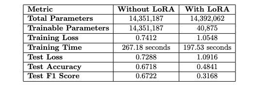
The finding revealed that while LoRA works well for larger models—where cutting down trainable parameters makes a big difference—the performance trade-off can be more pronounced in smaller models. TinyBERT, already tuned for fewer parameters, appeared to be more affected by the reductions from LoRA, leading to a significant decline in performance. This insight was crucial, indicating that the advantages of LoRA might significantly vary based on the model’s size and complexity during fine-tuning.

Key Insights and Reflections

1. Balancing Efficiency and Performance: A critical insight was balancing efficiency and performance. LoRA significantly lowers computational needs for fine-tuning, which is helpful in resource-limited settings. However, this efficiency slightly decreases accuracy. Understanding this trade-off is vital when choosing a fine-tuning approach.
2. Scalability Across Model Sizes: LoRA’s scalability across model sizes was a key takeaway. While effective for larger models like roberta-base, its impact on TinyBERT was complex, showing a significant accuracy drop. This suggests that LoRA may not suit models optimized for efficiency, highlighting the need to consider model architecture and size for parameter-efficient techniques in future projects.
3. Practical Implications for Real-World Applications: The experiments clarified LoRA’s practical implications. In settings with limited computational resources and training time, LoRA is a viable alternative to traditional fine-tuning, making it suitable for deploying large models where efficiency is crucial. However, in cases where accuracy is critical, such as medical diagnostics, the minor performance drop may be unacceptable, making standard fine-tuning a better choice.
   
   
   

Comparing Pretrained-Model Embedding

I further examined the potential of pre-trained models to generate embeddings for downstream tasks, particularly Visual Question Answering (VQA). I employed two configurations to extract embeddings: ResNet combined with SBERT (sentence-BERT) and CLIP (Contrastive Language-Image Pretraining). This process was distilled into a classification problem utilizing the DAQUAR dataset.

• ResNet-50 is a deep convolutional neural network (CNN) pre-trained on the ImageNet dataset, which contains millions of labeled images across thousands of classes. Using a pre-trained model like ResNet-50, we benefit from transfer learning, where the model’s ability to recognize and extract high-level image features can be leveraged for your specific task without retraining the entire model.
• SBERT (Sentence-BERT) is a variant of BERT (Bidirectional Encoder Representations from Transformers) designed to create sentence embeddings. SBERT is much faster than BERT when generating sentence embeddings, as it can produce dense, fixed-size representations of sentences or phrases that capture their semantic meaning.
• For tasks like Visual Question Answering, embeddings that understand the relationship between words in a sentence (e.g., a question) are essential. The particular version we used (all-MiniLM-L6-v2) is a lightweight transformer model optimized for performance with minimal loss in accuracy.
• The DAQUAR (DAtaset for QUestion Answering on Real-world images) dataset is designed for Visual Question Answering (VQA) tasks. It consists of real-world indoor scene images, where each image is paired with natural language questions and corresponding answers. The questions typically focus on objects in the scene, counting items, or identifying visual properties like color.

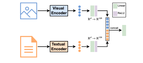
In the initial setup, I used ResNet-50 to generate image embeddings. The sentence transformer all-MiniLM-L6-v2 produced sentence embeddings. These image and text embeddings were merged and fed into a linear layer for classification.

The model consists of a linear layer utilizing ReLU activation for dimensionality reduction, followed by concatenating the processed embeddings. This combined representation is then input into a linear classifier. I trained the model and assessed its performance on the test set.

Here are the code snippets for this part:

1. Image Embedding Extraction using ResNet50:

from torchvision import models, transforms
import torch
from PIL import Image

# Load pretrained ResNet-50 wihtout the classification head
resnet = models.resnet50(pretraied=True)
resnet = torch.nn.Sequential(*list(resnet.childeren())[:-1])

# Image processing
transform = transforms.Compose{[
  transforms.Resize((224, 224)),
  transforms.ToTensor(),
  transforms.Normalize(mean=[0.485, 0.456, 0.406], std=0.229, 0.224, 0.225)
]}

# Extract image embedding
image = Image.open("path/to/image.jpg")
image = transform(image).unsqueeze(0)
with torch.no_grad():
    image_embedding = resnet(image).flatten()

• The mean and std values provided (mean=[0.485, 0.456, 0.406], std=[0.229, 0.224, 0.225]) are commonly used normalization values for image data. These values represent the channel-wise mean and standard deviation for the RGB channels (Red, Green, Blue) of images from the ImageNet dataset, which is used extensively to train many popular deep learning models, including ResNet.
• Embedding dimensionality (2048): The 2048-dimension embedding comes from the output of the last convolutional layer (before the fully connected layer, which is used for classification in the original model). This represents a compressed but detailed summary of the high-level features of the image. Each of the 2048 values corresponds to a particular feature learned by the model (e.g., edges, textures, or patterns).8.
  
  
  

2. Text Embeddings Extraction Using SBERT

from sentence_transformers import SentenceTransformer

sbert = SentenceTransformer('sentence-transformers/all-MiniLM-L6-v2')
text = "This is a sample question."
text_embedding = sbert.encode(text)

• Embedding dimensionality (384): The output embedding dimension of 384 from SBERT is a compact representation of the sentence’s meaning. The smaller dimensionality (compared to other BERT variants, which typically have 768 dimensions) makes it more computationally efficient while still retaining enough semantic detail for downstream tasks like classification.
  
  
  

3. Combining Image and Text Embeddings

We create a feature vector that blends visual and textual information by summing the embeddings. This combined embedding has a dimension of 2048 + 384, totaling 2432. However, this substantial embedding may include excessive details, leading to high computational costs for subsequent tasks, thus necessitating dimensionality reduction.

• Dimensionality Reduction to 512: To decrease the size of the merged embeddings, I implemented a linear layer to project the 2432-dimensional vector down to a more manageable 512-dimension . This approach mitigates computational complexity and helps prevent overfitting, mainly when training a classification model. The linear layer employs ReLU activation to efficiently reduce dimensionality while retaining the most vital features from both the image and text.

After training the model with the combined embeddings, I found that the test accuracy reached 0.3595 after 20 epochs. It was fascinating to see how merging visual and textual features created a richer representation of the input, which led to reasonably good results.

I will proceed with implementing CLIP to assess the performance of both models in the next post.