
Day97 Deep Learning Lecture Review - Lecture 15 (2)
Bias Mitigation Strategies: Loss Reweighting, Sampling & Synthetic Samples and Architectural Changes (OccamNets, Adversarial Training & DANN)

Four Main Strategies for Bias Mitigation
The lecture introduces several techniques aimed at mitigating bias in machine-learning models.
- Loss Reweighting
- Sampling
- Synthetic Samples
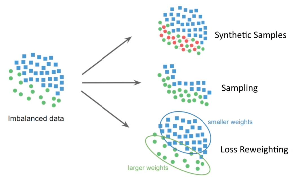
1. Sampling and Reweigting Methods
- Loss Reweighting
- We can re-weight the rarer samples during training for imbalanced datasets to make the system more robust.
- Assign higher loss weight for smaller populations.
- It requires to have co-variate labels.
- Often used for output labels.
- We can re-weight the rarer samples during training for imbalanced datasets to make the system more robust.
- Simple Sampling Strategies
- For each epoch, one could use any of these:
- Over-sample the smaller population.
- Under-sample the larger population.
- These methods allow the model to see samples from the minority population more often, so it is better learned.
- Sampling strategies are generally preferred over loss-based methods, especially in vision, where we use data augmentation.
- Two Choices:
- Epoch level: Identify the samples to use at the start of an epoch so that they are more balanced.
- Batch level: Ensure each mini-batch has the desired sample distribution so rarer subpopulations are present at the frequency we specify for each mini-batch.
- Hard Example Mining
- Rare samples often need to be more effectively learned by the model. We can leverage this to create mini-batches that help reduce bias without bias variables.
- Do a forward pass on $N$ samples and compute the loss on each one of them.
- Choose the $B$ samples with the highest loss for backprop, where $B<N$.
- Pottentially . such that high loss samples are more likely to be chosen.
- For each epoch, one could use any of these:
- Synthetic Minority Over-Sampling Technique (SMOTE)
- Only works on embeddings / vector data.
- Problem with sampling the original data is that it isn’t giving the system any real variety, so address that by creating synthetic (fake) embeddings.
- For minority samples, find their nearest neighbors from the same population.
- Create new samples that are the average of nearest neighbor pairs.
2. Robust Risk Minimization Methods for Bias Mitigations
Reduces the model’s reliance on spurious correlations and ensures it focuses on features generalizable across
-
Techniques
- Group DRO (Distributionally Robust Optimization)
- Used to find parameters that minimize the empirical worst-group risk.
- Enumerate all of your groups and find the parameters that minimize the worst-group training loss across groups.
- Method is very sensitive to hyperparameters.
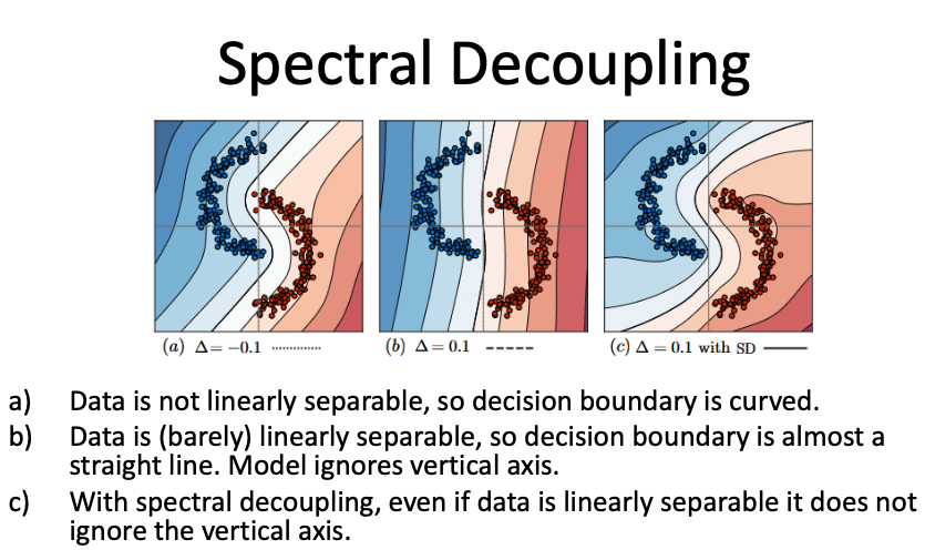
- Spectral Decoupling
- Spectral decoupling does not require bias variables and it aims to overcome bias by attacking gradient
starvation.
- Gradient Starvation: The tendency of the network to rely on statistically dominanat features (e.g., spurious variables) rather than all possible features.
- Penalizes the model for overly relying on features with high variance (spurious features).
- Encourages robustness by focusing on stable, core features across groups.
- Spectral decoupling does not require bias variables and it aims to overcome bias by attacking gradient
starvation.
- Group DRO (Distributionally Robust Optimization)
3. Architectural Changes
Incorporates inductive biases into model design to favor simpler, more generalizable solutions.
- Examples:
- OccamNets: Architectures designed to prioritize simpler solutions (aligns with Occam’s Razor).
- Adversarial Training:
- Adds adversarial examples to training to improve model robustness.
- Domain-Adversarial Neural Networks (DANN):
- Ensures features are invariant to specific domains or sensitive attributes like race or gender.
1. OccamNets
- Principle
- Inspired by Occam’s Razor, which suggests that simpler solutions are preferable unless complexity is justified by necessity. OccamNets are architectures designed to prioritize simplicity while maintaining predictive accuracy.
- How it works:
- Simpler hypothesis: OccamNets introduce constraints or priors in model architectures to discourage overfitting to complex patterns
- Regularization:
- Models incorporate penalties (e.g., $L_1$ or $L_2$ regularization) to limit the complexity of learned weights.
- Introduces inductive biases that favor simpler decision boundaries.
- Advantages:
- Enhances generalization: Models avoid fitting noise or spurious correlations in data.
- Reduces overfitting: Prevents models from relying on unnecessary complexities.
- Use case:
- Medical imaging: Ensures predictions rely on medically relevant features rather than noise or artifacts in images.
- Implementation techniques:
- Sparse architectures with dropouts.
- Regularization techniques like weight decay and sparsity constraints.
2. Adversarial Training
Image Source: Adversarial Machine Learning Mitigation: Adversarial Learning
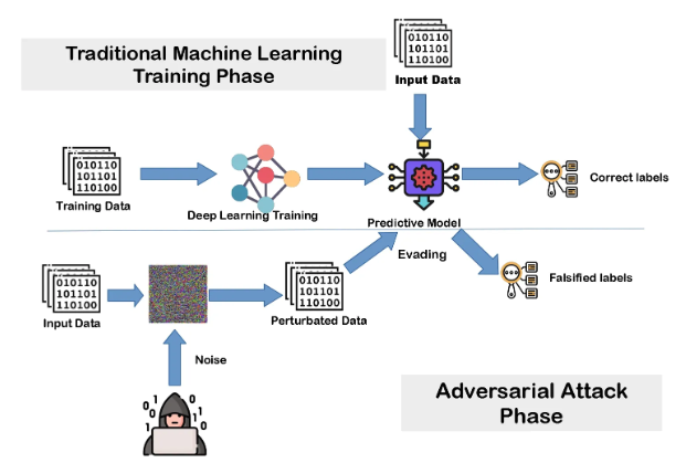
- Principle:
- Models can be susceptible to adversarial attacks—small perturbations in inputs that drastically change outputs. Adversarial training strengthens model robustness by incorporating adversarial examples in the training process.
-
How it works:
-
Adversarial example generation
- Small perturbations ($\delta$) are added to input data $x$ to maximize model loss
$x' = x + \delta, \quad \text{where } \delta = \epsilon \cdot \nabla_x \ell(f_\theta(x), y)$
- Here, $\epsilon$ controls the perturbation size, $\nabla_x$is the gradient, and $\ell$ is the loss.
-
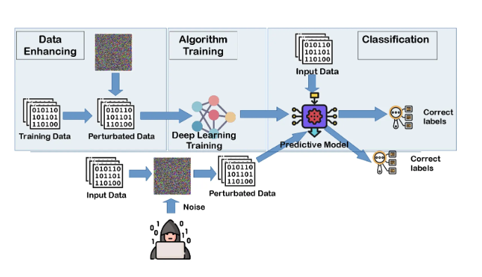
Training loop
- During each epoch, adversarial examples $x’$ are generated and included in training, making the model robust to these attacks.
-
- Benefits:
- Improves generalization to unseen data.
- Increases robustness to real-world noise and variations.
- Use case:
- Fraud detection: Models trained adversarially are less likely to be deceived by sophisticated fraud attempts.
- Challenges:
- Computationally expensive: Adversarial example generation increases training time.
- May not address all types of bias: Focused on robustness rather than fairness.
3. Domain-Adversarial Neural Networks (DANN)
- Principle:
- Ensures that features learned by a model are invariant across domains or sensitive attributes (e.g., race, gender). This is crucial for fair decision-making.
- How it works
- Network architecture
- Consists of three components:
- Feature extractor: Learns shared representations across domains.
- Label predictor: Predicts the primary target variable $Y$.
- Domain classifier: Predicts the domain or group $D$ from which the data originates.
- Adversarial objective:
- The feature extractor minimizes the loss for the label predictor while maximizing the loss for the domain classifier. This creates domain-invariant features:
- Consists of three components:
- Network architecture
$\text{Here, } \mathcal{L}_D \text{ is the domain classification loss, } \mathcal{L}_Y \text{ is the target classification loss, and } \lambda \text{ balances the tradeoff.} $
-
Benefits
- Mitigates bias from sensitive attributes by learning features that are independent of those attributes.
- Enhances fairness and robustness in multi-domain tasks.
-
Use case
- Hiring algorithms: Prevents models from leveraging features correlated with sensitive attributes like gender or race.
-
Challenges
- Performance tradeoff: Striving for domain invariance can slightly reduce performance on the main task.
- Performance tradeoff: Striving for domain invariance can slightly reduce performance on the main task.
When to Use These Techniques?
- OccamNets: Use when datasets have spurious correlations or when simpler, interpretable models are preferred.
- Adversarial Training: Use for applications where data or decisions can be adversarially manipulated (e.g., cybersecurity).
- DANN: Use for fairness-critical applications where biases related to sensitive domains need to be removed.
4. Example Code Snippets
1. OccamNets: Simplicity Through Regularization
Regularization is used to encourage simpler models by penalizing large weights.
-
Example Code: L1/L2 Regularization in PyTorch
import torch
import torch.nn as nn
import torch.optim as optim

# Define a simple neural network
class SimpleNet(nn.Module):
    def __init__(self):
        super(SimpleNet, self).__init__()
        self.fc1 = nn.Linear(10, 50)
        self.fc2 = nn.Linear(50, 1)

    def forward(self, x):
        x = torch.relu(self.fc1(x))
        x = self.fc2(x)
        return x

# Model and optimizer
model = SimpleNet()
optimizer = optim.Adam(model.parameters(), lr=0.001, weight_decay=1e-4)  # L2 regularization via weight_decay

# Training loop
criterion = nn.MSELoss()
for epoch in range(100):
    inputs = torch.randn(64, 10)  # Batch of inputs
    targets = torch.randn(64, 1)  # Batch of targets

    optimizer.zero_grad()
    outputs = model(inputs)
    loss = criterion(outputs, targets)
    loss.backward()
    optimizer.step()

    print(f"Epoch {epoch+1}, Loss: {loss.item()}")
Key Element:
weight_decay=1e-4applies L2 regularization, which penalizes large weights.
2. Adversarial Training
Adversarial training strengthens robustness by incorporating adversarial examples.
-
Example Code: Adversarial Training in PyTorch
import torch
import torch.nn as nn
import torch.optim as optim

# Define a simple neural network
class AdversarialNet(nn.Module):
    def __init__(self):
        super(AdversarialNet, self).__init__()
        self.fc1 = nn.Linear(10, 50)
        self.fc2 = nn.Linear(50, 1)

    def forward(self, x):
        x = torch.relu(self.fc1(x))
        x = self.fc2(x)
        return x

# Create adversarial example
def generate_adversarial_example(model, x, y, epsilon):
    x.requires_grad = True
    outputs = model(x)
    loss = nn.MSELoss()(outputs, y)
    model.zero_grad()
    loss.backward()
    x_adv = x + epsilon * x.grad.sign()
    return x_adv

# Model and optimizer
model = AdversarialNet()
optimizer = optim.Adam(model.parameters(), lr=0.001)

# Training loop with adversarial examples
for epoch in range(50):
    inputs = torch.randn(64, 10)
    targets = torch.randn(64, 1)

    # Generate adversarial examples
    adv_inputs = generate_adversarial_example(model, inputs, targets, epsilon=0.1)

    # Train on adversarial examples
    optimizer.zero_grad()
    outputs = model(adv_inputs)
    loss = nn.MSELoss()(outputs, targets)
    loss.backward()
    optimizer.step()

    print(f"Epoch {epoch+1}, Loss: {loss.item()}")
Key Element:
generate_adversarial_example()computes perturbations to inputs.
3. DANN: Domain-Adversarial Neural Networks
DANN ensures domain-invariant features by training a feature extractor adversarially against a domain classifier.
-
Example Code: Implementing DANN in PyTorch
import torch
import torch.nn as nn
import torch.optim as optim

# Define the feature extractor
class FeatureExtractor(nn.Module):
    def __init__(self):
        super(FeatureExtractor, self).__init__()
        self.fc1 = nn.Linear(10, 50)

    def forward(self, x):
        return torch.relu(self.fc1(x))

# Define the label predictor
class LabelPredictor(nn.Module):
    def __init__(self):
        super(LabelPredictor, self).__init__()
        self.fc = nn.Linear(50, 2)

    def forward(self, x):
        return torch.softmax(self.fc(x), dim=1)

# Define the domain classifier
class DomainClassifier(nn.Module):
    def __init__(self):
        super(DomainClassifier, self).__init__()
        self.fc = nn.Linear(50, 2)

    def forward(self, x):
        return torch.softmax(self.fc(x), dim=1)

# Instantiate models and optimizers
feature_extractor = FeatureExtractor()
label_predictor = LabelPredictor()
domain_classifier = DomainClassifier()

optimizer_F = optim.Adam(feature_extractor.parameters(), lr=0.001)
optimizer_L = optim.Adam(label_predictor.parameters(), lr=0.001)
optimizer_D = optim.Adam(domain_classifier.parameters(), lr=0.001)

# Training loop
for epoch in range(100):
    inputs = torch.randn(64, 10)  # Input data
    labels = torch.randint(0, 2, (64,))  # Task labels
    domains = torch.randint(0, 2, (64,))  # Domain labels

    # Feature extraction
    features = feature_extractor(inputs)

    # Task prediction loss
    predictions = label_predictor(features)
    loss_L = nn.CrossEntropyLoss()(predictions, labels)

    # Domain prediction loss (adversarial)
    domain_predictions = domain_classifier(features.detach())
    loss_D = nn.CrossEntropyLoss()(domain_predictions, domains)

    # Adversarial training
    optimizer_D.zero_grad()
    loss_D.backward()
    optimizer_D.step()

    optimizer_F.zero_grad()
    optimizer_L.zero_grad()
    (-loss_D + loss_L).backward()
    optimizer_F.step()
    optimizer_L.step()

    print(f"Epoch {epoch+1}, Task Loss: {loss_L.item()}, Domain Loss: {loss_D.item()}")
Key Element: The feature extractor is trained adversarially to confuse the domain classifier while optimizing task prediction.
Leave a comment